Figure 1: Cartoon of the enrichment of the mantle by a subduction slab.
This project is more numerically directed, with tests of algorithms for solving partial differential equations using finite difference schemes. Chapter 10 of the lecture notes provides the necessary theoretical background.
For this project you can collaborate with fellow students and you can hand in a common report. This project (together with projects 3 and 4) counts 1/3 of the final mark.
The project has a strong mathematical axis. However, for those interested, it should be straightforward to replace the dimensionless analysis in parts 5a-5f) with specific boundary and initial conditions. This is done in part 5g), with a focus on the heat equation and geophysical processes. That part is optional, but gives an additional 30 points to a score of 100.
The physical problem can be that of the temperature gradient in a rod of length \( L=1 \) or that of channel flow between two flat and infinite plates at \( x=0 \) and \( x=1 \), where the fluid is initially at rest and the plate \( x=1 \) is given a sudden initial movement. We are looking at a one-dimensional problem $$ \begin{equation*} \frac{\partial^2 u(x,t)}{\partial x^2} =\frac{\partial u(x,t)}{\partial t}, t> 0, x\in [0,L] \end{equation*} $$ or $$ \begin{equation*} u_{xx} = u_t, \end{equation*} $$ with initial conditions, i.e., the conditions at \( t=0 \), $$ \begin{equation*} u(x,0)= 0 \hspace{0.5cm} 0 < x < L \end{equation*} $$ with \( L=1 \) the length of the \( x \)-region of interest. The boundary conditions are $$ \begin{equation*} u(0,t)= 0 \hspace{0.5cm} t \ge 0, \end{equation*} $$ and $$ \begin{equation*} u(L,t)= 1 \hspace{0.5cm} t \ge 0. \end{equation*} $$ The function \( u(x,t) \) can be the temperature gradient of a rod or represent the fluid velocity in a direction parallel to the plates, that is normal to the \( x \)-axis. In the latter case, for small \( t \), only the part of the fluid close to the moving plate is set in significant motion, resulting in a thin boundary layer at \( x=1 \). As time increases, the velocity approaches a linear variation with \( x \). In this case, which can be derived from the incompressible Navier-Stokes, the above equations constitute a model for studying friction between moving surfaces separated by a thin fluid film.
In this project we want to study the numerical stability of three methods for partial differential equations (PDEs). These methods we will discuss are the explicit forward Euler algorithm with discretized versions of time given by a forward formula and a centered difference in space resulting in $$ \begin{equation*} u_t\approx \frac{u(x,t+\Delta t)-u(x,t)}{\Delta t}=\frac{u(x_i,t_j+\Delta t)-u(x_i,t_j)}{\Delta t} \end{equation*} $$ and $$ \begin{equation*} u_{xx}\approx \frac{u(x+\Delta x,t)-2u(x,t)+u(x-\Delta x,t)}{\Delta x^2}, \end{equation*} $$ or $$ \begin{equation*} u_{xx}\approx \frac{u(x_i+\Delta x,t_j)-2u(x_i,t_j)+u(x_i-\Delta x,t_j)}{\Delta x^2}. \end{equation*} $$ We will also discuss the implicit Backward Euler with $$ \begin{equation*} u_t\approx \frac{u(x,t)-u(x,t-\Delta t)}{\Delta t}=\frac{u(x_i,t_j)-u(x_i,t_j-\Delta t)}{\Delta t} \end{equation*} $$ and $$ \begin{equation*} u_{xx}\approx \frac{u(x+\Delta x,t)-2u(x,t)+u(x-\Delta x,t)}{\Delta x^2}, \end{equation*} $$ or $$ \begin{equation*} u_{xx}\approx \frac{u(x_i+\Delta x,t_j)-2u(x_i,t_j)+u(x_i-\Delta x,t_j)}{\Delta x^2}, \end{equation*} $$
Finally we use the implicit Crank-Nicolson scheme with a time-centered scheme at \( (x,t+\Delta t/2) \) $$ \begin{equation*} u_t\approx \frac{u(x,t+\Delta t)-u(x,t)}{\Delta t}=\frac{u(x_i,t_j+\Delta t)-u(x_i,t_j)}{\Delta t}. \end{equation*} $$ The corresponding spatial second-order derivative reads $$ \begin{align*} u_{xx}\approx &\frac{1}{2}\left(\frac{u(x_i+\Delta x,t_j)-2u(x_i,t_j)+u(x_i-\Delta x,t_j)}{\Delta x^2}\right. +\\ &\left. \frac{u(x_i+\Delta x,t_j+\Delta t)-2u(x_i,t_j+\Delta t)+u(x_i-\Delta x,t_j+\Delta t)}{\Delta x^2}\right). \end{align*} $$ Note well that we are using a time-centered scheme wih \( t+\Delta t/2 \) as center.
Here you can choose between an explicit or an implicit scheme. For the implicit scheme discussed in chapter 10 of the lecture notes, you need to use for example an iterative method like Jacobi's.
Outline the algorithm for solving the two-dimensional diffusion equation and implement the explicit or the implicit scheme as function of \( \Delta x \) (assuming \( \Delta x = \Delta y \)) and \( \Delta t \). Solve the equations numerically and give a critical discussion of your results. Compare your results with the closed-form answer. Discuss the stability of the solution as function of different values of \( \Delta x \) and \( \Delta t \).
You should, if you have time, try to parallelize the equations using MPI or OpenMP.
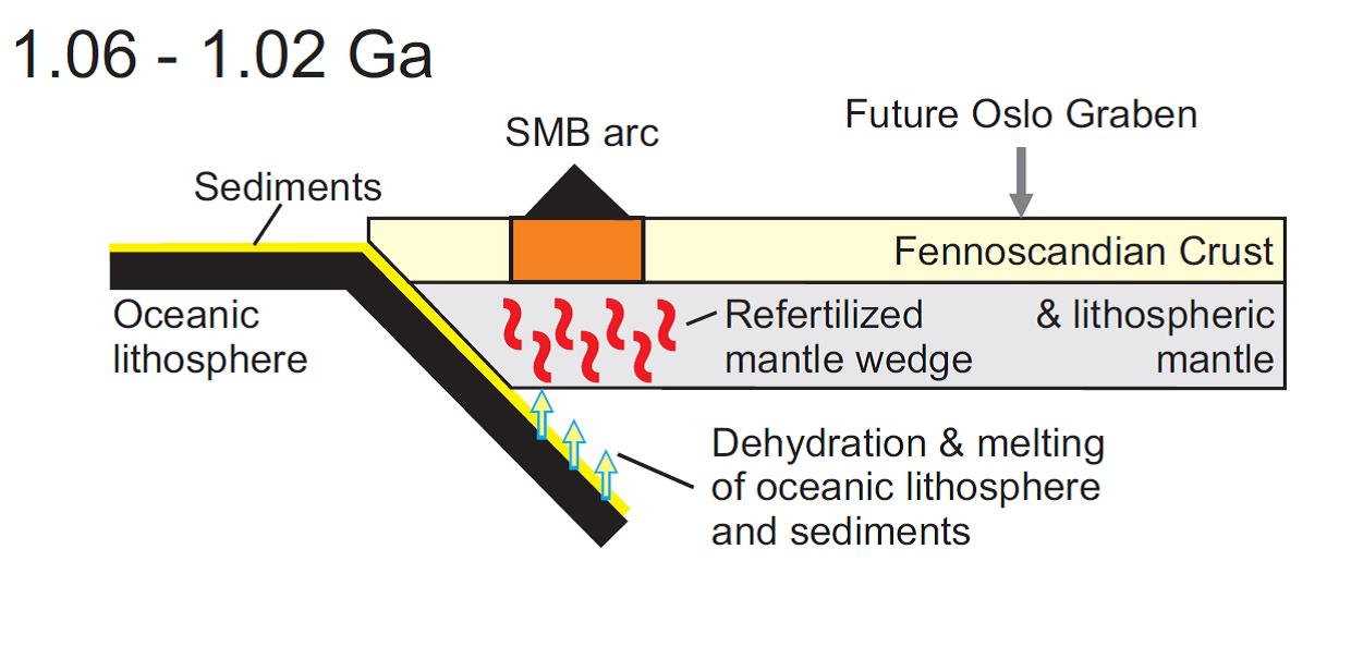
The Scientific background is based on geological evidence at the surface. Geologists have proposed that there was an active subduction zone on the western coast of Norway about 1Gy ago. When subducting, the oceanic lithosphere releases water and other chemical components that go mostly to the surface but may also be trapped in the mantle above the subducting slab. This process is called the refertilization of the mantle wedge (see Figure). These chemical components contain more radioactive elements than the normal mantle. We can therefore expect that ancient mantle wedges are enriched in radioactive elements and therefore warmer than normal mantle. The question is how much warmer they are and if we can find evidence for this enrichment in geophysical studies.
Figure 1: Cartoon of the enrichment of the mantle by a subduction slab.
The purpose of this part is to calculate the thermal evolution of the lithosphere up to present following the emplacement of radioactive elements in the mantle wedge 1 Gy ago.
The equation to compute is the time evolution of the temperature distribution is the heat equation, which will be used only in 2D here, namely $$ \begin{equation} \vec \nabla(k \vec \nabla T) + Q = \rho c_p \frac{\partial T}{\partial t} \label{eq:heat2D} \end{equation} $$ where \( T \) is the temperature, \( \rho \) is the density, \( k \) is the thermal conductivity, \( c_p \) is the specific heat capacity and \( Q \) is the heat production.
With the boundary conditions and initial conditions, you should rescale your equations in order to use the results from parts 5a-5f). The paramaters of the model are described here.
The boundary conditions are \( 8^{\circ}\,C \) at the surface and \( 1300^{\circ}C \) at the bottom at a depth of 120 km.
In this study, we assume a constant density for the lithosphere of \( 3.5 10^3\,Kg/m^3 \), a constant thermal conductivity of \( 2.5\,W/m/^{\circ}C \) and a constant specific heat capacity of \( 1000\,J/Kg/^{\circ}C^{-1} \).
The heat production, caused by radioactive decay, cannot be taken as uniform in the whole lithosphere as radioactive elements are much more abundant in the crust than in the mantle. We need therefore to separate the lithosphere in 3 units: the upper crust from 0 to 20 km depth, the lower crust from 20 to 40 km depth and the mantle from 40 to 120 km depth, where the heat production is set respectively to \( 1.4\,\mu W/m^3 \), \( 0.35\,\mu W/m^3 \) and \( 0.05\,\mu W/m^3 \).
Before radioactive enrichment, the temperature is steady-state and depends only on depth. In order to test your results you should try to obtain analytical results for the temperature profile as function of depth neglecting the presence of radioactice sources and. Compare thereafter these results with your numerical results. Include then the radioactive sources and compare eventual analytical results with numerical calculations.
We assume that the lithosphere above the slab gets enriched in radioactive elements U, Th and K 1 Gy ago and that this results in an additional heat production of \( 0.5\mu W/m^3 \) over the whole depth of the mantle (not the crust) in a 150 km wide area above the slab. Neglecting all other thermal perturbations that this slab could produce, and assuming that the heat production will remain constant over geological time, compute the thermal evolution of the lithosphere from 1 Gy to present.
The radioactivity will decrease with time. Assuming that the additional heat is produced at 40% by U, 40% by Th and 20% by K, which have halflives of 4.47 Gy, 14.0 Gy and 1.25 Gy respectively, compute the thermal evolution of the lithosphere and compare with the result obtained above.
A very good reference is the textbook by Winther and Tveito on partial differential equations. It is available online from the University library.
Here follows a brief recipe and recommendation on how to write a report for each project.
The preferred format for the report is a PDF file. You can also use DOC or postscript formats or as an ipython notebook file. As programming language we prefer that you choose between C/C++, Fortran2008 or Python. The following prescription should be followed when preparing the report: