
PHY321: Review of Vectors, Math and first Numerical Examples for simple Motion Problems
Morten Hjorth-Jensen, Department of Physics and Astronomy and National Superconducting Cyclotron Laboratory, Michigan State University, USA and Department of Physics, University of Oslo, Norway
Scott Pratt, Department of Physics and Astronomy and National Superconducting Cyclotron Laboratory, Michigan State University, USA
Carl Schmidt, Department of Physics and Astronomy, Michigan State University, USA
Date: Jan 14, 2020
Copyright 1999-2020, Morten Hjorth-Jensen. Released under CC Attribution-NonCommercial 4.0 license
Space, Time, Motion, Reference Frames and Reminder on vectors and other mathematical quantities
Our studies will start with the motion of different types of objects such as a falling ball, a runner, a bicycle etc etc. It means that an object's position in space varies with time. In order to study such systems we need to define
choice of origin
choice of the direction of the axes
choice of positive direction (left-handed or right-handed system of reference)
choice of units and dimensions
These choices lead to some important questions such as
is the physics of a system independent of the origin of the axes?
is the physics independent of the directions of the axes, that is are there privileged axes?
is the physics independent of the orientation of system?
is the physics independent of the scale of the length?
Dimension, units and labels
Throughout this course we will use the standardized SI units. The standard unit for length is thus one meter 1m, for mass one kilogram 1kg, for time one second 1s, for force one Newton 1kgm/s$^2$ and for energy 1 Joule 1kgm$^2$s$^{-2}$.
We will use the following notations for various variables (vectors are always boldfaced in these lecture notes):
position $\boldsymbol{r}$, in one dimention we will normally just use $x$,
mass $m$,
time $t$,
velocity $\boldsymbol{v}$ or just $v$ in one dimension,
acceleration $\boldsymbol{a}$ or just $a$ in one dimension,
momentum $\boldsymbol{p}$ or just $p$ in one dimension,
kinetic energy $K$,
potential energy $V$ and
frequency $\omega$.
More variables will be defined as we need them.
It is also important to keep track of dimensionalities. Don't mix this up with a chosen unit for a given variable. We mark the dimensionality in these lectures as $[a]$, where $a$ is the quantity we are interested in. Thus
$[\boldsymbol{r}]=$ length
$[m]=$ mass
$[K]=$ energy
$[t]=$ time
$[\boldsymbol{v}]=$ length over time
$[\boldsymbol{a}]=$ length over time squared
$[\boldsymbol{p}]=$ mass times length over time
$[\omega]=$ 1/time
Elements of Vector Algebra
Note: This section is under revision
In these lectures we will use boldfaced lower-case letters to label a vector. A vector $\boldsymbol{a}$ in three dimensions is thus defined as
$$ \boldsymbol{a} =(a_x,a_y, a_z), $$
and using the unit vectors in a cartesian system we have
$$ \boldsymbol{a} = a_x\boldsymbol{e}_x+a_y\boldsymbol{e}_y+a_z\boldsymbol{e}_z, $$
where the unit vectors have magnitude $\vert\boldsymbol{e}_i\vert = 1$ with $i=x,y,z$.
Using the fact that multiplication of reals is distributive we can show that
$$ \boldsymbol{a}(\boldsymbol{b}+\boldsymbol{c})=\boldsymbol{a}\boldsymbol{b}+\boldsymbol{a}\boldsymbol{c}, $$
Similarly we can also show that (using product rule for differentiating reals)
$$ \frac{d}{dt}(\boldsymbol{a}\boldsymbol{b})=\boldsymbol{a}\frac{d\boldsymbol{b}}{dt}+\boldsymbol{b}\frac{d\boldsymbol{a}}{dt}. $$
We can repeat these operations for the cross products and show that they are distribuitive
$$ \boldsymbol{a}\times(\boldsymbol{b}+\boldsymbol{c})=\boldsymbol{a}\times\boldsymbol{b}+\boldsymbol{a}\times\boldsymbol{c}. $$
We have also that
$$ \frac{d}{dt}(\boldsymbol{a}\times\boldsymbol{b})=\boldsymbol{a}\times\frac{d\boldsymbol{b}}{dt}+\boldsymbol{b}\times\frac{d\boldsymbol{a}}{dt}. $$
The rotation of a three-dimensional vector $\boldsymbol{a}=(a_x,a_y,a_z)$ in the $xy$ plane around an angle $\phi$ results in a new vector $\boldsymbol{b}=(b_x,b_y,b_z)$. This operation can be expressed in terms of linear algebra as a matrix (the rotation matrix) multiplied with a vector. We can write this as
$$ \begin{bmatrix} b_x \\ b_y \\ b_z \end{bmatrix} = \begin{bmatrix} \cos{\phi} & \sin{\phi} & 0 \\ -\sin{\phi} & \cos{\phi} & 0 \\ 0 & 0 & 1\end{bmatrix}\begin{bmatrix} a_x \\ a_y \\ a_z \end{bmatrix}. $$
We can write this in a more compact form as $\boldsymbol{b} = \boldsymbol{R}\boldsymbol{a}$, where the rotation matrix is defined as
$$ \boldsymbol{R} = \begin{bmatrix} \cos{\phi} & \sin{\phi} & 0 \\ -\sin{\phi} & \cos{\phi} & 0 \\ 0 & 0 & 1\end{bmatrix}. $$
Falling baseball in one dimension
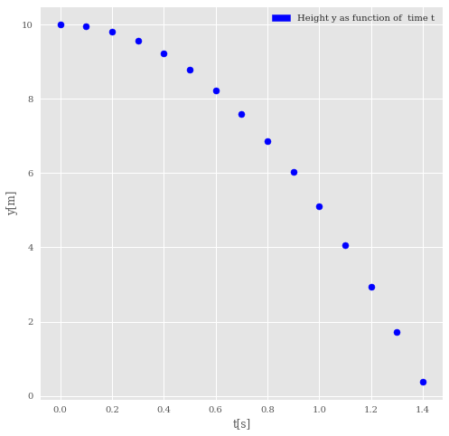
We anticipate the mathematical model to come and assume that we have a model for the motion of a falling baseball without air resistance. Our system (the baseball) is at an initial height $y_0$ (which we will specify in the program below) at the initial time $t_0=0$. In our program example here we will plot the position in steps of $\Delta t$ up to a final time $t_f$. The mathematical formula for the position $y(t)$ as function of time $t$ is
$$ y(t) = y_0-\frac{1}{2}gt^2, $$
where $g=9.80665=0.980655\times 10^1$m/s${}^2$ is a constant representing the standard acceleration due to gravity. We have here adopted the conventional standard value. This does not take into account other effects, such as buoyancy or drag. Furthermore, we stop when the ball hits the ground, which takes place at
$$ y(t) = 0= y_0-\frac{1}{2}gt^2, $$
which gives us a final time $t_f=\sqrt{2y_0/g}$.
As of now we simply assume that we know the formula for the falling object. Afterwards, we will derive it.
Our Python Encounter
We start with preparing folders for storing our calculations, figures and if needed, specific data files we use as input or output files.
%matplotlib inline

# Common imports
import numpy as np
import pandas as pd
import matplotlib.pyplot as plt
import os

# Where to save the figures and data files
PROJECT_ROOT_DIR = "Results"
FIGURE_ID = "Results/FigureFiles"
DATA_ID = "DataFiles/"

if not os.path.exists(PROJECT_ROOT_DIR):
    os.mkdir(PROJECT_ROOT_DIR)

if not os.path.exists(FIGURE_ID):
    os.makedirs(FIGURE_ID)

if not os.path.exists(DATA_ID):
    os.makedirs(DATA_ID)

def image_path(fig_id):
    return os.path.join(FIGURE_ID, fig_id)

def data_path(dat_id):
    return os.path.join(DATA_ID, dat_id)

def save_fig(fig_id):
    plt.savefig(image_path(fig_id) + ".png", format='png')

#in case we have an input file we wish to read in
#infile = open(data_path("MassEval2016.dat"),'r')
You could also define a function for making our plots. You can obviously avoid this and simply set up various matplotlib commands every time you need them. You may however find it convenient to collect all such commands in one function and simply call this function.
from pylab import plt, mpl
plt.style.use('seaborn')
mpl.rcParams['font.family'] = 'serif'

def MakePlot(x,y, styles, labels, axlabels):
    plt.figure(figsize=(10,6))
    for i in range(len(x)):
        plt.plot(x[i], y[i], styles[i], label = labels[i])
        plt.xlabel(axlabels[0])
        plt.ylabel(axlabels[1])
    plt.legend(loc=0)
Thereafter we start setting up the code for the falling object.
%matplotlib inline
import matplotlib.patches as mpatches

g = 9.80655 #m/s^2
y_0 = 10.0 # initial position in meters
DeltaT = 0.1  # time step
# final time when y = 0, t = sqrt(2*10/g)
tfinal = np.sqrt(2.0*y_0/g)
#set up arrays
t = np.arange(0,tfinal,DeltaT)
y =y_0 -g*.5*t**2
# Then make a nice printout in table form using Pandas
import pandas as pd
from IPython.display import display
data = {'t[s]': t,
        'y[m]': y
        }
RawData = pd.DataFrame(data)
display(RawData)
plt.style.use('ggplot')
plt.figure(figsize=(8,8))
plt.scatter(t, y, color = 'b')
blue_patch = mpatches.Patch(color = 'b', label = 'Height y as function of  time t')
plt.legend(handles=[blue_patch])
plt.xlabel("t[s]")
plt.ylabel("y[m]")
save_fig("FallingBaseball")
plt.show()
$$ \overline{v}(t) = \frac{y(t+\Delta t)-y(t)}{\Delta t}. $$
In the code we have set the time step $\Delta t$ to a given value. We could define it in terms of the number of points $n$ as
$$ \Delta t = \frac{t_{\mathrm{final}-}t_{\mathrm{initial}}}{n+1}. $$
Since we have discretized the variables, we introduce the counter $i$ and let $y(t)\rightarrow y(t_i)=y_i$ and $t\rightarrow t_i$ with $i=0,1,\dots, n$. This gives us the following shorthand notations that we will use for the rest of this course. We define
$$ y_i = y(t_i),\hspace{0.2cm} i=0,1,2,\dots,n. $$
This applies to other variables which depend on say time. Examples are the velocities, accelerations, momenta etc. Furthermore we use the shorthand
$$ y_{i\pm 1} = y(t_i\pm \Delta t),\hspace{0.12cm} i=0,1,2,\dots,n. $$
$$ \overline{v}_i = \frac{y_{i+1}-y_{i}}{\Delta t}. $$
The velocity is defined as the change in position per unit time. In the limit $\Delta t \rightarrow 0$ this defines the instantaneous velocity, which is nothing but the slope of the position at a time $t$. We have thus
$$ v(t) = \frac{dy}{dt}=\lim_{\Delta t \rightarrow 0}\frac{y(t+\Delta t)-y(t)}{\Delta t}. $$
Similarly, we can define the average acceleration as the change in velocity per unit time as
$$ \overline{a}_i = \frac{v_{i+1}-v_{i}}{\Delta t}, $$
resulting in the instantaneous acceleration
$$ a(t) = \frac{dv}{dt}=\lim_{\Delta t\rightarrow 0}\frac{v(t+\Delta t)-v(t)}{\Delta t}. $$
$$ a(t) = \frac{dv}{dt}=\frac{d}{dt}\frac{dy}{dt}=\frac{d^2y}{dt^2}. $$
This forms the starting point for our definition of forces later. It is a famous second-order differential equation. If the acceleration is constant we can now recover the formula for the falling ball we started with. The acceleration can depend on the position and the velocity. To be more formal we should then write the above differential equation as
$$ \frac{d^2y}{dt^2}=a(t,y(t),\frac{dy}{dt}). $$
With given initial conditions for $y(t_0)$ and $v(t_0)$ we can then integrate the above equation and find the velocities and positions at a given time $t$.
If we multiply with mass, we have one of the famous expressions for Newton's second law,
$$ F(y,v,t)=m\frac{d^2y}{dt^2}=ma(t,y(t),\frac{dy}{dt}), $$
where $F$ is the force acting on an object with mass $m$. We see that it also has the right dimension, mass times length divided by time squared. We will come back to this soon.
Integrating our equations
Formally we can then, starting with the acceleration (suppose we have measured it, how could we do that?) compute say the height of a building. To see this we perform the following integrations from an initial time $t_0$ to a given time $t$
$$ \int_{t_0}^t dt a(t) = \int_{t_0}^t dt \frac{dv}{dt} = v(t)-v(t_0), $$
or as
$$ v(t)=v(t_0)+\int_{t_0}^t dt a(t). $$
When we know the velocity as function of time, we can find the position as function of time starting from the defintion of velocity as the derivative with respect to time, that is we have
$$ \int_{t_0}^t dt v(t) = \int_{t_0}^t dt \frac{dy}{dt} = y(t)-y(t_0), $$
or as
$$ y(t)=y(t_0)+\int_{t_0}^t dt v(t). $$
These equations define what is called the integration method for finding the position and the velocity as functions of time. There is no loss of generality if we extend these equations to more than one spatial dimension.
Constant acceleration case, the velocity
Let us compute the velocity using the constant value for the acceleration given by $-g$. We have
$$ v(t)=v(t_0)+\int_{t_0}^t dt a(t)=v(t_0)+\int_{t_0}^t dt (-g). $$
Using our initial time as $t_0=0$s and setting the initial velocity $v(t_0)=v_0=0$m/s we get when integrating
$$ v(t)=-gt. $$
The more general case is
$$ v(t)=v_0-g(t-t_0). $$
We can then integrate the velocity and obtain the final formula for the position as function of time through
$$ y(t)=y(t_0)+\int_{t_0}^t dt v(t)=y_0+\int_{t_0}^t dt v(t)=y_0+\int_{t_0}^t dt (-gt), $$
With $y_0=10$m and $t_0=0$s, we obtain the equation we started with
$$ y(t)=10-\frac{1}{2}gt^2. $$
# Now we can compute the mean velocity using our data
# We define first an array Vaverage
n = np.size(t)
Vaverage = np.zeros(n)
for i in range(1,n-1):
    Vaverage[i] = (y[i+1]-y[i])/DeltaT
# Now we can compute the mean accelearatio using our data
# We define first an array Aaverage
n = np.size(t)
Aaverage = np.zeros(n)
Aaverage[0] = -g
for i in range(1,n-1):
    Aaverage[i] = (Vaverage[i+1]-Vaverage[i])/DeltaT
data = {'t[s]': t,
        'y[m]': y,
        'v[m/s]': Vaverage,
        'a[m/s^2]': Aaverage
        }
NewData = pd.DataFrame(data)
display(NewData[0:n-2])
Note that we don't print the last values!
Including Air Resistance in our model
In our discussions till now of the falling baseball, we have ignored air resistance and simply assumed that our system is only influenced by the gravitational force. We will postpone the derivation of air resistance till later, after our discussion of Newton's laws and forces.
For our discussions here it suffices to state that the accelerations is now modified to
$$ \boldsymbol{a}(t) = -g +D\boldsymbol{v}(t)\vert v(t)\vert, $$
where $\vert v(t)\vert$ is the absolute value of the velocity and $D$ is a constant which pertains to the specific object we are studying. Since we are dealing with motion in one dimension, we can simplify the above to
$$ a(t) = -g +Dv^2(t). $$
We can rewrite this as a differential equation
$$ a(t) = \frac{dv}{dt}=\frac{d^2y}{dt^2}= -g +Dv^2(t). $$
Using the integral equations discussed above we can integrate twice and obtain first the velocity as function of time and thereafter the position as function of time.
For this particular case, we can actually obtain an analytical solution for the velocity and for the position. Here we will first compute the solutions analytically, thereafter we will derive Euler's method for solving these differential equations numerically.
Analytical solutions
For simplicity let us just write $v(t)$ as $v$. We have
$$ \frac{dv}{dt}= -g +Dv^2(t). $$
We can solve this using the technique of separation of variables. We isolate on the left all terms that involve $v$ and on the right all terms that involve time. We get then
$$ \frac{dv}{g -Dv^2(t) }= -dt, $$
We scale now the equation to the left by introducing a constant $v_T=\sqrt{g/D}$. This constant has dimension length/time. Can you show this?
Next we integrate the left-hand side (lhs) from $v_0=0$ m/s to $v$ and the right-hand side (rhs) from $t_0=0$ to $t$ and obtain
$$ \int_{0}^v\frac{dv}{g -Dv^2(t) }= \frac{v_T}{g}\mathrm{arctanh}(\frac{v}{v_T}) =-\int_0^tdt = -t. $$
We can reorganize these equations as
$$ v_T\mathrm{arctanh}(\frac{v}{v_T}) =-gt, $$
which gives us $v$ as function of time
$$ v(t)=v_T\tanh{-(\frac{gt}{v_T})}. $$
$$ y(t)=y(t_0)+\int_{t_0}^t dt v(t)=\int_{0}^t dt[v_T\tanh{-(\frac{gt}{v_T})}]. $$
This integral is a little bit trickier but we can look it up in a table over known integrals and we get
$$ y(t)=y(t_0)-\frac{v_T^2}{g}\log{[\cosh{(\frac{gt}{v_T})}]}. $$
Alternatively we could have used the symbolic Python package Sympy (example will be inserted later).
In most cases however, we need to revert to numerical solutions.
Our first attempt at solving differential equations
Here we will try the simplest possible approach to solving the second-order differential equation
$$ a(t) =\frac{d^2y}{dt^2}= -g +Dv^2(t). $$
We rewrite it as two coupled first-order equations (this is a standard approach)
$$ \frac{dy}{dt} = v(t), $$
with initial condition $y(t_0)=y_0$ and
$$ a(t) =\frac{dv}{dt}= -g +Dv^2(t), $$
with initial condition $v(t_0)=v_0$.
Many of the algorithms for solving differential equations start with simple Taylor equations. If we now Taylor expand $y$ and $v$ around a value $t+\Delta t$ we have
$$ y(t+\Delta t) = y(t)+\Delta t \frac{dy}{dt}+\frac{\Delta t^2}{2!} \frac{d^2y}{dt^2}+O(\Delta t^3), $$
and
$$ v(t+\Delta t) = v(t)+\Delta t \frac{dv}{dt}+\frac{\Delta t^2}{2!} \frac{d^2v}{dt^2}+O(\Delta t^3). $$
Using the fact that $dy/dt = v$ and $dv/dt=a$ and keeping only terms up to $\Delta t$ we have
$$ y(t+\Delta t) = y(t)+\Delta t v(t)+O(\Delta t^2), $$
and
$$ v(t+\Delta t) = v(t)+\Delta t a(t)+O(\Delta t^2). $$
$$ y_{i+1} = y_i+\Delta t v_i, $$
and
$$ v_{i+1} = v_i+\Delta t a_i. $$
These are the famous Euler equations (forward Euler).
To solve these equations numerically we start at a time $t_0$ and simply integrate up these equations to a final time $t_f$, The step size $\Delta t$ is an input parameter in our code. You can define it directly in the code below as
DeltaT = 0.1
With a given final time tfinal we can then find the number of integration points via the ceil function included in the math package of Python as
#define final time, assuming that initial time is zero
from math import ceil
tfinal = 0.5
n = ceil(tfinal/DeltaT)
print(n)
The ceil function returns the smallest integer not less than the input in say
x = 21.15
print(ceil(x))
which in the case here is 22.
x = 21.75
print(ceil(x))
which also yields 22. The floor function in the math package is used to return the closest integer value which is less than or equal to the specified expression or value. Compare the previous result to the usage of floor
from math import floor
x = 21.75
print(floor(x))
Alternatively, we can define ourselves the number of integration(mesh) points. In this case we could have
n = 10
tinitial = 0.0
tfinal = 0.5
DeltaT = (tfinal-tinitial)/(n)
print(DeltaT)
Since we will set up one-dimensional arrays that contain the values of various variables like time, position, velocity, acceleration etc, we need to know the value of $n$, the number of data points (or integration or mesh points). With $n$ we can initialize a given array by setting all elelements to zero, as done here
# define array a
a = np.zeros(n)
print(a)
# Common imports
import numpy as np
import pandas as pd
from math import *
import matplotlib.pyplot as plt
import os

# Where to save the figures and data files
PROJECT_ROOT_DIR = "Results"
FIGURE_ID = "Results/FigureFiles"
DATA_ID = "DataFiles/"

if not os.path.exists(PROJECT_ROOT_DIR):
    os.mkdir(PROJECT_ROOT_DIR)

if not os.path.exists(FIGURE_ID):
    os.makedirs(FIGURE_ID)

if not os.path.exists(DATA_ID):
    os.makedirs(DATA_ID)

def image_path(fig_id):
    return os.path.join(FIGURE_ID, fig_id)

def data_path(dat_id):
    return os.path.join(DATA_ID, dat_id)

def save_fig(fig_id):
    plt.savefig(image_path(fig_id) + ".png", format='png')


g = 9.80655 #m/s^2
D = 0.00245 #m/s
DeltaT = 0.1
#set up arrays
tfinal = 0.5
n = ceil(tfinal/DeltaT)
# define scaling constant vT
vT = sqrt(g/D)
# set up arrays for t, a, v, and y and we can compare our results with analytical ones
t = np.zeros(n)
a = np.zeros(n)
v = np.zeros(n)
y = np.zeros(n)
yanalytic = np.zeros(n)
# Initial conditions
v[0] = 0.0  #m/s
y[0] = 10.0 #m
yanalytic[0] = y[0]
# Start integrating using Euler's method
for i in range(n-1):
    # expression for acceleration
    a[i] = -g + D*v[i]*v[i]
    # update velocity and position
    y[i+1] = y[i] + DeltaT*v[i]
    v[i+1] = v[i] + DeltaT*a[i]
    # update time to next time step and compute analytical answer
    t[i+1] = t[i] + DeltaT
    yanalytic[i+1] = y[0]-(vT*vT/g)*log(cosh(g*t[i+1]/vT))
    if ( y[i+1] < 0.0):
        break
a[n-1] = -g + D*v[n-1]*v[n-1]
data = {'t[s]': t,
        'y[m]': y-yanalytic,
        'v[m/s]': v,
        'a[m/s^2]': a
        }
NewData = pd.DataFrame(data)
display(NewData)
#finally we plot the data
fig, axs = plt.subplots(3, 1)
axs[0].plot(t, y, t, yanalytic)
axs[0].set_xlim(0, tfinal)
axs[0].set_ylabel('y and exact')
axs[1].plot(t, v)
axs[1].set_ylabel('v[m/s]')
axs[2].plot(t, a)
axs[2].set_xlabel('time[s]')
axs[2].set_ylabel('a[m/s^2]')
fig.tight_layout()
save_fig("EulerIntegration")
plt.show()
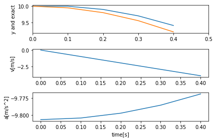
Try different values for $\Delta t$ and study the difference between the exact solution and the numerical solution.
Simple extension, the Euler-Cromer method
The Euler-Cromer method is a simple variant of the standard Euler method. We use the newly updated velocity $v_{i+1}$ as an input to the new position, that is, instead of
$$ y_{i+1} = y_i+\Delta t v_i, $$
and
$$ v_{i+1} = v_i+\Delta t a_i, $$
we use now the newly calculate for $v_{i+1}$ as input to $y_{i+1}$, that is we compute first
$$ v_{i+1} = v_i+\Delta t a_i, $$
and then
$$ y_{i+1} = y_i+\Delta t v_{i+1}, $$
Implementing the Euler-Cromer method yields a simple change to the previous code. We only need to change the following line in the loop over time steps
for i in range(n-1):
    # more codes in between here
    v[i+1] = v[i] + DeltaT*a[i]
    y[i+1] = y[i] + DeltaT*v[i+1]
    # more code
Python practicalities, Software and needed installations
We will make extensive use of Python as programming language and its myriad of available libraries. You will find Jupyter notebooks invaluable in your work.
If you have Python installed (we strongly recommend Python3) and you feel pretty familiar with installing different packages, we recommend that you install the following Python packages via pip as
- pip install numpy scipy matplotlib ipython scikit-learn mglearn sympy pandas pillow
For Python3, replace pip with pip3.
For OSX users we recommend, after having installed Xcode, to install brew. Brew allows for a seamless installation of additional software via for example
- brew install python3
For Linux users, with its variety of distributions like for example the widely popular Ubuntu distribution, you can use pip as well and simply install Python as
- sudo apt-get install python3 (or python for pyhton2.7)
etc etc.
Python installers
If you don't want to perform these operations separately and venture into the hassle of exploring how to set up dependencies and paths, we recommend two widely used distrubutions which set up all relevant dependencies for Python, namely
which is an open source distribution of the Python and R programming languages for large-scale data processing, predictive analytics, and scientific computing, that aims to simplify package management and deployment. Package versions are managed by the package management system conda.
is a Python distribution for scientific and analytic computing distribution and analysis environment, available for free and under a commercial license.
Furthermore, Google's Colab is a free Jupyter notebook environment that requires no setup and runs entirely in the cloud. Try it out!
Useful Python libraries
Here we list several useful Python libraries we strongly recommend (if you use anaconda many of these are already there)
NumPy is a highly popular library for large, multi-dimensional arrays and matrices, along with a large collection of high-level mathematical functions to operate on these arrays
The pandas library provides high-performance, easy-to-use data structures and data analysis tools
Xarray is a Python package that makes working with labelled multi-dimensional arrays simple, efficient, and fun!
Scipy (pronounced “Sigh Pie”) is a Python-based ecosystem of open-source software for mathematics, science, and engineering.
Matplotlib is a Python 2D plotting library which produces publication quality figures in a variety of hardcopy formats and interactive environments across platforms.
Autograd can automatically differentiate native Python and Numpy code. It can handle a large subset of Python's features, including loops, ifs, recursion and closures, and it can even take derivatives of derivatives of derivatives
SymPy is a Python library for symbolic mathematics.
scikit-learn has simple and efficient tools for machine learning, data mining and data analysis
TensorFlow is a Python library for fast numerical computing created and released by Google
Keras is a high-level neural networks API, written in Python and capable of running on top of TensorFlow, CNTK, or Theano
Your jupyter notebook can easily be converted into a nicely rendered PDF file or a Latex file for further processing. For example, convert to latex as
pycod jupyter nbconvert filename.ipynb --to latex And to add more versatility, the Python package SymPy is a Python library for symbolic mathematics. It aims to become a full-featured computer algebra system (CAS) and is entirely written in Python.
Numpy examples and Important Matrix and vector handling packages
There are several central software libraries for linear algebra and eigenvalue problems. Several of the more popular ones have been wrapped into ofter software packages like those from the widely used text Numerical Recipes. The original source codes in many of the available packages are often taken from the widely used software package LAPACK, which follows two other popular packages developed in the 1970s, namely EISPACK and LINPACK. We describe them shortly here.
LINPACK: package for linear equations and least square problems.
LAPACK:package for solving symmetric, unsymmetric and generalized eigenvalue problems. From LAPACK's website http://www.netlib.org it is possible to download for free all source codes from this library. Both C/C++ and Fortran versions are available.
BLAS (I, II and III): (Basic Linear Algebra Subprograms) are routines that provide standard building blocks for performing basic vector and matrix operations. Blas I is vector operations, II vector-matrix operations and III matrix-matrix operations. Highly parallelized and efficient codes, all available for download from http://www.netlib.org.
Basic Matrix Features
Matrix properties reminder.
$$ \mathbf{A} = \begin{bmatrix} a_{11} & a_{12} & a_{13} & a_{14} \\ a_{21} & a_{22} & a_{23} & a_{24} \\ a_{31} & a_{32} & a_{33} & a_{34} \\ a_{41} & a_{42} & a_{43} & a_{44} \end{bmatrix}\qquad \mathbf{I} = \begin{bmatrix} 1 & 0 & 0 & 0 \\ 0 & 1 & 0 & 0 \\ 0 & 0 & 1 & 0 \\ 0 & 0 & 0 & 1 \end{bmatrix} $$
The inverse of a matrix is defined by
$$ \mathbf{A}^{-1} \cdot \mathbf{A} = I $$
| Relations | Name | matrix elements |
|---|---|---|
| $A = A^{T}$ | symmetric | $a_{ij} = a_{ji}$ |
| $A = \left (A^{T} \right )^{-1}$ | real orthogonal | $\sum_k a_{ik} a_{jk} = \sum_k a_{ki} a_{kj} = \delta_{ij}$ |
| $A = A^{ * }$ | real matrix | $a_{ij} = a_{ij}^{ * }$ |
| $A = A^{\dagger}$ | hermitian | $a_{ij} = a_{ji}^{ * }$ |
| $A = \left (A^{\dagger} \right )^{-1}$ | unitary | $\sum_k a_{ik} a_{jk}^{ * } = \sum_k a_{ki}^{ * } a_{kj} = \delta_{ij}$ |
Some famous Matrices
Diagonal if $a_{ij}=0$ for $i\ne j$
Upper triangular if $a_{ij}=0$ for $i > j$
Lower triangular if $a_{ij}=0$ for $i < j$
Upper Hessenberg if $a_{ij}=0$ for $i > j+1$
Lower Hessenberg if $a_{ij}=0$ for $i < j+1$
Tridiagonal if $a_{ij}=0$ for $|i -j| > 1$
Lower banded with bandwidth $p$: $a_{ij}=0$ for $i > j+p$
Upper banded with bandwidth $p$: $a_{ij}=0$ for $i < j+p$
Banded, block upper triangular, block lower triangular....
More Basic Matrix Features
Some Equivalent Statements.
For an $N\times N$ matrix $\mathbf{A}$ the following properties are all equivalent
If the inverse of $\mathbf{A}$ exists, $\mathbf{A}$ is nonsingular.
The equation $\mathbf{Ax}=0$ implies $\mathbf{x}=0$.
The rows of $\mathbf{A}$ form a basis of $R^N$.
The columns of $\mathbf{A}$ form a basis of $R^N$.
$\mathbf{A}$ is a product of elementary matrices.
$0$ is not eigenvalue of $\mathbf{A}$.
Numpy and arrays
Numpy provides an easy way to handle arrays in Python. The standard way to import this library is as
import numpy as np
Here follows a simple example where we set up an array of ten elements, all determined by random numbers drawn according to the normal distribution,
n = 10
x = np.random.normal(size=n)
print(x)
We defined a vector $x$ with $n=10$ elements with its values given by the Normal distribution $N(0,1)$. Another alternative is to declare a vector as follows
import numpy as np
x = np.array([1, 2, 3])
print(x)
Here we have defined a vector with three elements, with $x_0=1$, $x_1=2$ and $x_2=3$. Note that both Python and C++ start numbering array elements from $0$ and on. This means that a vector with $n$ elements has a sequence of entities $x_0, x_1, x_2, \dots, x_{n-1}$. We could also let (recommended) Numpy to compute the logarithms of a specific array as
import numpy as np
x = np.log(np.array([4, 7, 8]))
print(x)
In the last example we used Numpy's unary function $np.log$. This function is highly tuned to compute array elements since the code is vectorized and does not require looping. We normaly recommend that you use the Numpy intrinsic functions instead of the corresponding log function from Python's math module. The looping is done explicitely by the np.log function. The alternative, and slower way to compute the logarithms of a vector would be to write
import numpy as np
from math import log
x = np.array([4, 7, 8])
for i in range(0, len(x)):
    x[i] = log(x[i])
print(x)
We note that our code is much longer already and we need to import the log function from the math module. The attentive reader will also notice that the output is $[1, 1, 2]$. Python interprets automagically our numbers as integers (like the automatic keyword in C++). To change this we could define our array elements to be double precision numbers as
import numpy as np
x = np.log(np.array([4, 7, 8], dtype = np.float64))
print(x)
or simply write them as double precision numbers (Python uses 64 bits as default for floating point type variables), that is
import numpy as np
x = np.log(np.array([4.0, 7.0, 8.0])
print(x)
To check the number of bytes (remember that one byte contains eight bits for double precision variables), you can use simple use the itemsize functionality (the array $x$ is actually an object which inherits the functionalities defined in Numpy) as
import numpy as np
x = np.log(np.array([4.0, 7.0, 8.0])
print(x.itemsize)
import numpy as np
A = np.log(np.array([ [4.0, 7.0, 8.0], [3.0, 10.0, 11.0], [4.0, 5.0, 7.0] ]))
print(A)
If we use the shape function we would get $(3, 3)$ as output, that is verifying that our matrix is a $3\times 3$ matrix. We can slice the matrix and print for example the first column (Python organized matrix elements in a row-major order, see below) as
import numpy as np
A = np.log(np.array([ [4.0, 7.0, 8.0], [3.0, 10.0, 11.0], [4.0, 5.0, 7.0] ]))
# print the first column, row-major order and elements start with 0
print(A[:,0])
We can continue this was by printing out other columns or rows. The example here prints out the second column
import numpy as np
A = np.log(np.array([ [4.0, 7.0, 8.0], [3.0, 10.0, 11.0], [4.0, 5.0, 7.0] ]))
# print the first column, row-major order and elements start with 0
print(A[1,:])
Numpy contains many other functionalities that allow us to slice, subdivide etc etc arrays. We strongly recommend that you look up the Numpy website for more details. Useful functions when defining a matrix are the np.zeros function which declares a matrix of a given dimension and sets all elements to zero
import numpy as np
n = 10
# define a matrix of dimension 10 x 10 and set all elements to zero
A = np.zeros( (n, n) )
print(A)
or initializing all elements to
import numpy as np
n = 10
# define a matrix of dimension 10 x 10 and set all elements to one
A = np.ones( (n, n) )
print(A)
or as unitarily distributed random numbers (see the material on random number generators in the statistics part)
import numpy as np
n = 10
# define a matrix of dimension 10 x 10 and set all elements to random numbers with x \in [0, 1]
A = np.random.rand(n, n)
print(A)
Meet the Pandas

Another useful Python package is pandas, which is an open source library providing high-performance, easy-to-use data structures and data analysis tools for Python. pandas stands for panel data, a term borrowed from econometrics and is an efficient library for data analysis with an emphasis on tabular data. pandas has two major classes, the DataFrame class with two-dimensional data objects and tabular data organized in columns and the class Series with a focus on one-dimensional data objects. Both classes allow you to index data easily as we will see in the examples below. pandas allows you also to perform mathematical operations on the data, spanning from simple reshapings of vectors and matrices to statistical operations.
The following simple example shows how we can, in an easy way make tables of our data. Here we define a data set which includes names, place of birth and date of birth, and displays the data in an easy to read way. We will see repeated use of pandas, in particular in connection with classification of data.
import pandas as pd
from IPython.display import display
data = {'First Name': ["Frodo", "Bilbo", "Aragorn II", "Samwise"],
        'Last Name': ["Baggins", "Baggins","Elessar","Gamgee"],
        'Place of birth': ["Shire", "Shire", "Eriador", "Shire"],
        'Date of Birth T.A.': [2968, 2890, 2931, 2980]
        }
data_pandas = pd.DataFrame(data)
display(data_pandas)
In the above we have imported pandas with the shorthand pd, the latter has become the standard way we import pandas. We make then a list of various variables and reorganize the above lists into a DataFrame and then print out a neat table with specific column labels as Name, place of birth and date of birth. Displaying these results, we see that the indices are given by the default numbers from zero to three. pandas is extremely flexible and we can easily change the above indices by defining a new type of indexing as
data_pandas = pd.DataFrame(data,index=['Frodo','Bilbo','Aragorn','Sam'])
display(data_pandas)
Thereafter we display the content of the row which begins with the index Aragorn
display(data_pandas.loc['Aragorn'])
We can easily append data to this, for example
new_hobbit = {'First Name': ["Peregrin"],
              'Last Name': ["Took"],
              'Place of birth': ["Shire"],
              'Date of Birth T.A.': [2990]
              }
data_pandas=data_pandas.append(pd.DataFrame(new_hobbit, index=['Pippin']))
display(data_pandas)
Here are other examples where we use the DataFrame functionality to handle arrays, now with more interesting features for us, namely numbers. We set up a matrix of dimensionality $10\times 5$ and compute the mean value and standard deviation of each column. Similarly, we can perform mathematial operations like squaring the matrix elements and many other operations.
import numpy as np
import pandas as pd
from IPython.display import display
np.random.seed(100)
# setting up a 10 x 5 matrix
rows = 10
cols = 5
a = np.random.randn(rows,cols)
df = pd.DataFrame(a)
display(df)
print(df.mean())
print(df.std())
display(df**2)
Thereafter we can select specific columns only and plot final results
df.columns = ['First', 'Second', 'Third', 'Fourth', 'Fifth']
df.index = np.arange(10)

display(df)
print(df['Second'].mean() )
print(df.info())
print(df.describe())

from pylab import plt, mpl
plt.style.use('seaborn')
mpl.rcParams['font.family'] = 'serif'

df.cumsum().plot(lw=2.0, figsize=(10,6))
plt.show()


df.plot.bar(figsize=(10,6), rot=15)
plt.show()
We can produce a $4\times 4$ matrix
b = np.arange(16).reshape((4,4))
print(b)
df1 = pd.DataFrame(b)
print(df1)
and many other operations.
The Series class is another important class included in pandas. You can view it as a specialization of DataFrame but where we have just a single column of data. It shares many of the same features as _DataFrame. As with DataFrame, most operations are vectorized, achieving thereby a high performance when dealing with computations of arrays, in particular labeled arrays. As we will see below it leads also to a very concice code close to the mathematical operations we may be interested in. For multidimensional arrays, we recommend strongly xarray. xarray has much of the same flexibility as pandas, but allows for the extension to higher dimensions than two.