Deep Learning: Project 2 and Convolutional Neural Networks

Plans for week 7 and week 8

Second project

Possible paths for project 2

We discuss here several paths as well as data sets for the second project

1. The computational path: Here we propose a path where you develop your own code for a neural networks (or CNNs or RNNs) and apply this to data of your own selection. The code should be object oriented and flexible allowing for eventual extensions by including different Loss/Cost functions and other functionalities. Feel free to select data sets from those suggested below here. This code can also be extended upon by adding for example autoencoders. You can compare your own codes with implementations using TensorFlow(Keras)/PyTorch or other libraries.
2. The differential equation path: Here we propose a set of differential equations (ordinary and/or partial) to be solved first using neural networks (using either your own code or TensorFlow/Pytorch or similar libraries). Thereafter we plan to extend the set of methods for solving these equations to recurrent neural networks and autoencoders. All these approaches can be expanded into one large project. This project can also be extended into including Physics informed machine learning. Here we can discuss neural networks that are trained to solve supervised learning tasks while respecting any given law of physics described by general nonlinear partial differential equations.
3. The application path: Here you can use the most relevant method(s) (say neural networks, convolutional neural networks for images) and apply this(these) to data sets relevant for your own research.
4. And finally we propose also a partial differential equation path.

You can propose own data sets that relate to your research interests or just use existing data sets from say

1. Kaggle
2. The University of California at Irvine (UCI) with its machine learning repository.
3. For the differential equation problems, you can generate your own datasets, as described below.
4. If possible, you should link the data sets with existing research and analyses thereof. Scientific articles which have used Machine Learning algorithms to analyze the data are highly welcome. Perhaps you can improve previous analyses and even publish a new article?
5. A critical assessment of the methods with ditto perspectives and recommendations is also something you need to include.

The approach to the analysis of these new data sets should follow to a large extent what you did in project 1. That is:

1. Whether you end up with a regression or a classification problem, you should employ at least two of the methods we have discussed among linear regression (including Ridge and Lasso), Logistic Regression, Neural Networks, Convolution Neural Networks, Recurrent Neural Networks, Adversarial Neural Networks, Support Vector Machines and Decision Trees, Random Forests, Bagging and Boosting.
2. The estimates you used and tested in project 1 should also be included, that is the \( R2 \)-score, MSE, confusion matrix, accuracy score, information gain, ROC and Cumulative gains curves and other, cross-validation and/or bootstrap if these are relevant.
3. Similarly, feel free to explore various activations functions in deep learning and various approachs to stochastic gradient descent approaches.

All in all, the report should follow the same pattern as project 1, with abstract, introduction, methods, code, results, conclusions etc.

Solving differential equations with neural networks

Here we describe the possible differential equations we can study first with neural networks and thereafter with recurrent neural networks and/or AE and/or GANs.

The differential equations are given by the so-called Lorenz attractor model, and read

 
$$ \frac{dx}{dt}=\sigma\left(y-x\right), $$

where \( \sigma =10 \) is a constant

 
$$ \frac{dy}{dt}= x\left(\rho-z\right)-y, $$

with \( \rho=28 \) and

 
$$ \frac{dz}{dt}=xy-\beta z $$

with \( \beta=8/3 \) as our final constant.

The following function is a simple function which sets up the solution using the ordinary differential library which follows NumPy. Here we have fixed the time sted \( \Delta t=0.01 \) and the final time \( t_f=8 \).

The program sets \( 100 \) random initial values and produces inputs and outputs for a neural network calculations. The inputs are given by the values of the array \( \boldsymbol{x} \) (which contains \( x,y,z \) as functions of time) for the time step \( \boldsymbol{x}_t \). The other array defined by \( \boldsymbol{x}_{t+1} \) contains the outputs (or targets) which we want the neural network to reproduce.

# Common imports
import numpy as np
from scipy.integrate import odeint
import matplotlib.pyplot as plt
import os

# Where to save the figures and data files
PROJECT_ROOT_DIR = "Results"
FIGURE_ID = "Results/FigureFiles"
DATA_ID = "DataFiles/"

if not os.path.exists(PROJECT_ROOT_DIR):
    os.mkdir(PROJECT_ROOT_DIR)

if not os.path.exists(FIGURE_ID):
    os.makedirs(FIGURE_ID)

if not os.path.exists(DATA_ID):
    os.makedirs(DATA_ID)

def image_path(fig_id):
    return os.path.join(FIGURE_ID, fig_id)

def data_path(dat_id):
    return os.path.join(DATA_ID, dat_id)

def save_fig(fig_id):
    plt.savefig(image_path(fig_id) + ".png", format='png')


# Selection of parameter values and setting array for time
dt =0.01; tfinal = 8
t = np.arange(0,tfinal+dt, dt)
beta =8.0/3.0; rho = 28.0; sigma = 10.0

# define the inputs and outputs for the neural networks
nninput = np.zeros((100*len(t)-1,3))
nnoutput = np.zeros((100*len(t)-1,3))
# Define the equations to integrate
def lorenz_derivative(xyz, t0, sigma=sigma,beta=beta,rho=rho):
    x, y, z = xyz
    return [sigma*(x-y), x*(rho-z)-y, x*y-beta*z]

# generate 100 random initial values
x0 = -15.0+30.0*np.random.random((100,3))

# Use odeint functionality by sending in derivative function
# Feel free to change the choice of integrator
x_t = np.asarray([odeint(lorenz_derivative, x0_j, t) 
                  for x0_j in x0])

# define the inputs and outputs for the neural networks
for j in range(100):
    nninput[j*(len(t)-1):(j+1)*(len(t)-1),:] = x_t[j,:-1,:]
    nnoutput[j*(len(t)-1):(j+1)*(len(t)-1),:] = x_t[j,1:,:]

The input and output variables are those we will start trying our network with. Your first taks is to set up a neural code (either using your own code or TensorFlow/PyTorch or similar libraries)) and use the above data to a prediction for the time evolution of Lorenz system for various values of the randomly chosen initial values. Study the dependence of the fit as function of the architecture of the network (number of nodes, hidden layers and types of activation functions) and various regularization schemes and optimization methods like standard gradient descent with momentum, stochastic gradient descent with batches and with and without momentum and various schedulers for the learning rate.

Feel free to change the above differential equations. As an example, consider the following harmonic oscillator equations solved with the Runge-Kutta to fourth order method. This is a one-dimensional problem and it produces a position \( x_t \) and velocity \( v_t \). You could now try to fit both the velocities and positions using much of the same recipe as for Lorenz attractor. You will find it convenient to analyze one set of initial conditions first. The code is included here.

This code is an example code that solves Newton's equations of motion with a given force and produces an output which in turn can be used to train a neural network

# Common imports
import numpy as np
import pandas as pd
from math import *
import matplotlib.pyplot as plt
import os

# Where to save the figures and data files
PROJECT_ROOT_DIR = "Results"
FIGURE_ID = "Results/FigureFiles"
DATA_ID = "DataFiles/"

if not os.path.exists(PROJECT_ROOT_DIR):
    os.mkdir(PROJECT_ROOT_DIR)

if not os.path.exists(FIGURE_ID):
    os.makedirs(FIGURE_ID)

if not os.path.exists(DATA_ID):
    os.makedirs(DATA_ID)

def image_path(fig_id):
    return os.path.join(FIGURE_ID, fig_id)

def data_path(dat_id):
    return os.path.join(DATA_ID, dat_id)

def save_fig(fig_id):
    plt.savefig(image_path(fig_id) + ".png", format='png')


def SpringForce(v,x,t):
#   note here that we have divided by mass and we return the acceleration
    return  -2*gamma*v-x+Ftilde*cos(t*Omegatilde)


def RK4(v,x,t,n,Force):
    for i in range(n-1):
# Setting up k1
        k1x = DeltaT*v[i]
        k1v = DeltaT*Force(v[i],x[i],t[i])
# Setting up k2
        vv = v[i]+k1v*0.5
        xx = x[i]+k1x*0.5
        k2x = DeltaT*vv
        k2v = DeltaT*Force(vv,xx,t[i]+DeltaT*0.5)
# Setting up k3
        vv = v[i]+k2v*0.5
        xx = x[i]+k2x*0.5
        k3x = DeltaT*vv
        k3v = DeltaT*Force(vv,xx,t[i]+DeltaT*0.5)
# Setting up k4
        vv = v[i]+k3v
        xx = x[i]+k3x
        k4x = DeltaT*vv
        k4v = DeltaT*Force(vv,xx,t[i]+DeltaT)
# Final result
        x[i+1] = x[i]+(k1x+2*k2x+2*k3x+k4x)/6.
        v[i+1] = v[i]+(k1v+2*k2v+2*k3v+k4v)/6.
        t[i+1] = t[i] + DeltaT


# Main part begins here

DeltaT = 0.001
#set up arrays 
tfinal = 20 # in dimensionless time
n = ceil(tfinal/DeltaT)
# set up arrays for t, v, and x
t = np.zeros(n)
v = np.zeros(n)
x = np.zeros(n)
# Initial conditions (can change to more than one dim)
x0 =  1.0 
v0 = 0.0
x[0] = x0
v[0] = v0
gamma = 0.2
Omegatilde = 0.5
Ftilde = 1.0
# Start integrating using Euler's method
# Note that we define the force function as a SpringForce
RK4(v,x,t,n,SpringForce)

# Plot position as function of time    
fig, ax = plt.subplots()
ax.set_ylabel('x[m]')
ax.set_xlabel('t[s]')
ax.plot(t, x)
fig.tight_layout()
save_fig("ForcedBlockRK4")
plt.show()

The next step is to include recurrent neural networks. These will be discussed in connection with coming lectures.

Finally we add a so-called differential equation path as well.

Solving partial differential equations with neural networks

For this variant of project 2, we will assume that you have some background in the solution of partial differential equations using finite difference schemes. In the lecture slides from weeks 6 and 7 you may find additional material. We will study the solution of the diffusion equation in one dimension using a standard explicit or implicit scheme and neural networks to solve the same equations.

For the explicit and/or implicit schemes, you can study for example chapter 10 of the lecture notes in Computational Physics or alternative sources.

For the machine learning part you can use the functionality of for example Tensorflow/Keras.

Part a), setting up the problem

The physical problem can be that of the temperature gradient in a rod of length \( L=1 \) at \( x=0 \) and \( x=1 \). We are looking at a one-dimensional problem

 
$$ \begin{equation*} \frac{\partial^2 u(x,t)}{\partial x^2} =\frac{\partial u(x,t)}{\partial t}, t> 0, x\in [0,L] \end{equation*} $$

or

 
$$ \begin{equation*} u_{xx} = u_t, \end{equation*} $$

with initial conditions, i.e., the conditions at \( t=0 \),

 
$$ \begin{equation*} u(x,0)= \sin{(\pi x)} \hspace{0.5cm} 0 < x < L, \end{equation*} $$

with \( L=1 \) the length of the \( x \)-region of interest. The boundary conditions are

 
$$ \begin{equation*} u(0,t)= 0 \hspace{0.5cm} t \ge 0, \end{equation*} $$

and

 
$$ \begin{equation*} u(L,t)= 0 \hspace{0.5cm} t \ge 0. \end{equation*} $$

The function \( u(x,t) \) can be the temperature gradient of a rod. As time increases, the velocity approaches a linear variation with \( x \).

We will limit ourselves to the so-called explicit forward Euler algorithm with discretized versions of time given by a forward formula and a centered difference in space resulting in

 
$$ \begin{equation*} u_t\approx \frac{u(x,t+\Delta t)-u(x,t)}{\Delta t}=\frac{u(x_i,t_j+\Delta t)-u(x_i,t_j)}{\Delta t} \end{equation*} $$

and

 
$$ \begin{equation*} u_{xx}\approx \frac{u(x+\Delta x,t)-2u(x,t)+u(x-\Delta x,t)}{\Delta x^2}, \end{equation*} $$

or

 
$$ \begin{equation*} u_{xx}\approx \frac{u(x_i+\Delta x,t_j)-2u(x_i,t_j)+u(x_i-\Delta x,t_j)}{\Delta x^2}. \end{equation*} $$

Write down the algorithm and the equations you need to implement. Find also the analytical solution to the problem.

Part b)

Implement the explicit scheme algorithm and perform tests of the solution for \( \Delta x=1/10 \), \( \Delta x=1/100 \) using \( \Delta t \) as dictated by the stability limit of the explicit scheme. The stability criterion for the explicit scheme requires that \( \Delta t/\Delta x^2 \leq 1/2 \).

Study the solutions at two time points \( t_1 \) and \( t_2 \) where \( u(x,t_1) \) is smooth but still significantly curved and \( u(x,t_2) \) is almost linear, close to the stationary state.

Part c) Neural networks

Study now the lecture notes on solving ODEs and PDEs with neural network and use either your own code or the functionality of tensorflow/keras to solve the same equation as in part b). Discuss your results and compare them with the standard explicit or implicit scheme. Include also the analytical solution and compare with that.

Part d)

Finally, present a critical assessment of the methods you have studied and discuss the potential for the solving differential equations and eigenvalue problems with machine learning methods.

Convolutional Neural Networks (recognizing images)

Convolutional neural networks (CNNs) were developed during the last decade of the previous century, with a focus on character recognition tasks. Nowadays, CNNs are a central element in the spectacular success of deep learning methods. The success in for example image classifications have made them a central tool for most machine learning practitioners.

CNNs are very similar to ordinary Neural Networks. They are made up of neurons that have learnable weights and biases. Each neuron receives some inputs, performs a dot product and optionally follows it with a non-linearity. The whole network still expresses a single differentiable score function: from the raw image pixels on one end to class scores at the other. And they still have a loss function (for example Softmax) on the last (fully-connected) layer and all the tips/tricks we developed for learning regular Neural Networks still apply (back propagation, gradient descent etc etc).

What is the Difference

CNN architectures make the explicit assumption that the inputs are images, which allows us to encode certain properties into the architecture. These then make the forward function more efficient to implement and vastly reduce the amount of parameters in the network.

Here we provide only a superficial overview, for the more interested, we recommend highly the course IN5400 – Machine Learning for Image Analysis and the slides of CS231.

Another good read is the article here https://arxiv.org/pdf/1603.07285.pdf.

Neural Networks vs CNNs

Neural networks are defined as affine transformations, that is a vector is received as input and is multiplied with a matrix of so-called weights (our unknown paramters) to produce an output (to which a bias vector is usually added before passing the result through a nonlinear activation function). This is applicable to any type of input, be it an image, a sound clip or an unordered collection of features: whatever their dimensionality, their representation can always be flattened into a vector before the transformation.

Why CNNS for images, sound files, medical images from CT scans etc?

However, when we consider images, sound clips and many other similar kinds of data, these data have an intrinsic structure. More formally, they share these important properties:

• They are stored as multi-dimensional arrays (think of the pixels of a figure) .
• They feature one or more axes for which ordering matters (e.g., width and height axes for an image, time axis for a sound clip).
• One axis, called the channel axis, is used to access different views of the data (e.g., the red, green and blue channels of a color image, or the left and right channels of a stereo audio track).

These properties are not exploited when an affine transformation is applied; in fact, all the axes are treated in the same way and the topological information is not taken into account. Still, taking advantage of the implicit structure of the data may prove very handy in solving some tasks, like computer vision and speech recognition, and in these cases it would be best to preserve it. This is where discrete convolutions come into play.

A discrete convolution is a linear transformation that preserves this notion of ordering. It is sparse (only a few input units contribute to a given output unit) and reuses parameters (the same weights are applied to multiple locations in the input).

Regular NNs don’t scale well to full images

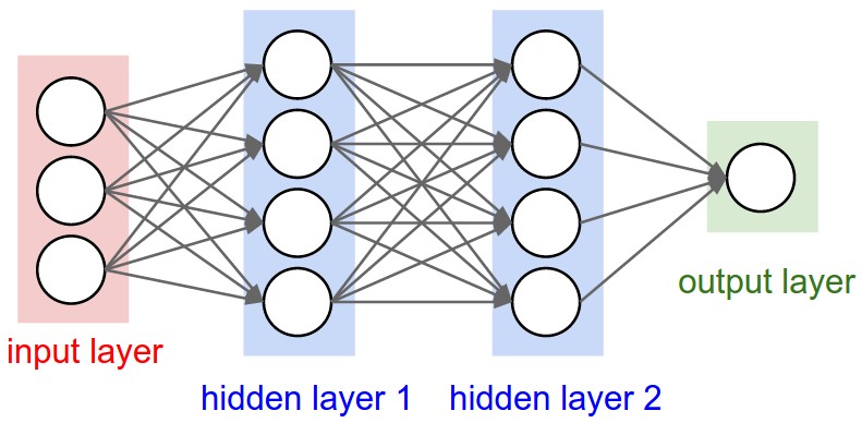
As an example, consider an image of size \( 32\times 32\times 3 \) (32 wide, 32 high, 3 color channels), so a single fully-connected neuron in a first hidden layer of a regular Neural Network would have \( 32\times 32\times 3 = 3072 \) weights. This amount still seems manageable, but clearly this fully-connected structure does not scale to larger images. For example, an image of more respectable size, say \( 200\times 200\times 3 \), would lead to neurons that have \( 200\times 200\times 3 = 120,000 \) weights.

We could have several such neurons, and the parameters would add up quickly! Clearly, this full connectivity is wasteful and the huge number of parameters would quickly lead to possible overfitting.

3D volumes of neurons

Convolutional Neural Networks take advantage of the fact that the input consists of images and they constrain the architecture in a more sensible way.

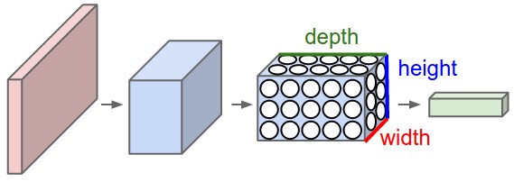
In particular, unlike a regular Neural Network, the layers of a CNN have neurons arranged in 3 dimensions: width, height, depth. (Note that the word depth here refers to the third dimension of an activation volume, not to the depth of a full Neural Network, which can refer to the total number of layers in a network.)

To understand it better, the above example of an image with an input volume of activations has dimensions \( 32\times 32\times 3 \) (width, height, depth respectively).

The neurons in a layer will only be connected to a small region of the layer before it, instead of all of the neurons in a fully-connected manner. Moreover, the final output layer could for this specific image have dimensions \( 1\times 1 \times 10 \), because by the end of the CNN architecture we will reduce the full image into a single vector of class scores, arranged along the depth dimension.

Layers used to build CNNs

A simple CNN is a sequence of layers, and every layer of a CNN transforms one volume of activations to another through a differentiable function. We use three main types of layers to build CNN architectures: Convolutional Layer, Pooling Layer, and Fully-Connected Layer (exactly as seen in regular Neural Networks). We will stack these layers to form a full CNN architecture.

A simple CNN for image classification could have the architecture:

• INPUT (\( 32\times 32 \times 3 \)) will hold the raw pixel values of the image, in this case an image of width 32, height 32, and with three color channels R,G,B.
• CONV (convolutional )layer will compute the output of neurons that are connected to local regions in the input, each computing a dot product between their weights and a small region they are connected to in the input volume. This may result in volume such as \( [32\times 32\times 12] \) if we decided to use 12 filters.
• RELU layer will apply an elementwise activation function, such as the \( max(0,x) \) thresholding at zero. This leaves the size of the volume unchanged (\( [32\times 32\times 12] \)).
• POOL (pooling) layer will perform a downsampling operation along the spatial dimensions (width, height), resulting in volume such as \( [16\times 16\times 12] \).
• FC (i.e. fully-connected) layer will compute the class scores, resulting in volume of size \( [1\times 1\times 10] \), where each of the 10 numbers correspond to a class score, such as among the 10 categories of the MNIST images we considered above . As with ordinary Neural Networks and as the name implies, each neuron in this layer will be connected to all the numbers in the previous volume.

Transforming images

CNNs transform the original image layer by layer from the original pixel values to the final class scores.

Observe that some layers contain parameters and other don’t. In particular, the CNN layers perform transformations that are a function of not only the activations in the input volume, but also of the parameters (the weights and biases of the neurons). On the other hand, the RELU/POOL layers will implement a fixed function. The parameters in the CONV/FC layers will be trained with gradient descent so that the class scores that the CNN computes are consistent with the labels in the training set for each image.

CNNs in brief

In summary:

• A CNN architecture is in the simplest case a list of Layers that transform the image volume into an output volume (e.g. holding the class scores)
• There are a few distinct types of Layers (e.g. CONV/FC/RELU/POOL are by far the most popular)
• Each Layer accepts an input 3D volume and transforms it to an output 3D volume through a differentiable function
• Each Layer may or may not have parameters (e.g. CONV/FC do, RELU/POOL don’t)
• Each Layer may or may not have additional hyperparameters (e.g. CONV/FC/POOL do, RELU doesn’t)

For more material on convolutional networks, we strongly recommend the course IN5400 – Machine Learning for Image Analysis and the slides of CS231 which is taught at Stanford University (consistently ranked as one of the top computer science programs in the world). Michael Nielsen's book is a must read, in particular chapter 6 which deals with CNNs.

The textbook by Goodfellow et al, see chapter 9 contains an in depth discussion as well.

Key Idea

A dense neural network is representd by an affine operation (like matrix-matrix multiplication) where all parameters are included.

The key idea in CNNs for say imaging is that in images neighbor pixels tend to be related! So we connect only neighboring neurons in the input instead of connecting all with the first hidden layer.

We say we perform a filtering (convolution is the mathematical operation).

Mathematics of CNNs

The mathematics of CNNs is based on the mathematical operation of convolution. In mathematics (in particular in functional analysis), convolution is represented by mathematical operation (integration, summation etc) on two function in order to produce a third function that expresses how the shape of one gets modified by the other. Convolution has a plethora of applications in a variety of disciplines, spanning from statistics to signal processing, computer vision, solutions of differential equations,linear algebra, engineering, and yes, machine learning.

Mathematically, convolution is defined as follows (one-dimensional example): Let us define a continuous function \( y(t) \) given by

 
$$ y(t) = \int x(a) w(t-a) da, $$

where \( x(a) \) represents a so-called input and \( w(t-a) \) is normally called the weight function or kernel.

The above integral is written in a more compact form as

 
$$ y(t) = \left(x * w\right)(t). $$

The discretized version reads

 
$$ y(t) = \sum_{a=-\infty}^{a=\infty}x(a)w(t-a). $$

Computing the inverse of the above convolution operations is known as deconvolution.

How can we use this? And what does it mean? Let us study some familiar examples first.

Convolution Examples: Polynomial multiplication

We have already met such an example in project 1 when we tried to set up the design matrix for a two-dimensional function. This was an example of polynomial multiplication. Let us recast such a problem in terms of the convolution operation. Let us look a the following polynomials to second and third order, respectively:

 
$$ p(t) = \alpha_0+\alpha_1 t+\alpha_2 t^2, $$

and

 
$$ s(t) = \beta_0+\beta_1 t+\beta_2 t^2+\beta_3 t^3. $$

The polynomial multiplication gives us a new polynomial of degree \( 5 \)

 
$$ z(t) = \delta_0+\delta_1 t+\delta_2 t^2+\delta_3 t^3+\delta_4 t^4+\delta_5 t^5. $$

Efficient Polynomial Multiplication

Computing polynomial products can be implemented efficiently if we rewrite the more brute force multiplications using convolution. We note first that the new coefficients are given as

 
$$ \begin{split} \delta_0=&\alpha_0\beta_0\\ \delta_1=&\alpha_1\beta_0+\alpha_1\beta_0\\ \delta_2=&\alpha_0\beta_2+\alpha_1\beta_1+\alpha_2\beta_0\\ \delta_3=&\alpha_1\beta_2+\alpha_2\beta_1+\alpha_0\beta_3\\ \delta_4=&\alpha_2\beta_2+\alpha_1\beta_3\\ \delta_5=&\alpha_2\beta_3.\\ \end{split} $$

We note that \( \alpha_i=0 \) except for \( i\in \left\{0,1,2\right\} \) and \( \beta_i=0 \) except for \( i\in\left\{0,1,2,3\right\} \).

We can then rewrite the coefficients \( \delta_j \) using a discrete convolution as

 
$$ \delta_j = \sum_{i=-\infty}^{i=\infty}\alpha_i\beta_{j-i}=(\alpha * \beta)_j, $$

or as a double sum with restriction \( l=i+j \)

 
$$ \delta_l = \sum_{ij}\alpha_i\beta_{j}. $$

Do you see a potential drawback with these equations?

A more efficient way of coding the above Convolution

Since we only have a finite number of \( \alpha \) and \( \beta \) values which are non-zero, we can rewrite the above convolution expressions as a matrix-vector multiplication

 
$$ \boldsymbol{\delta}=\begin{bmatrix}\alpha_0 & 0 & 0 & 0 \\ \alpha_1 & \alpha_0 & 0 & 0 \\ \alpha_2 & \alpha_1 & \alpha_0 & 0 \\ 0 & \alpha_2 & \alpha_1 & \alpha_0 \\ 0 & 0 & \alpha_2 & \alpha_1 \\ 0 & 0 & 0 & \alpha_2 \end{bmatrix}\begin{bmatrix} \beta_0 \\ \beta_1 \\ \beta_2 \\ \beta_3\end{bmatrix}. $$

The process is commutative and we can easily see that we can rewrite the multiplication in terms of a matrix holding \( \beta \) and a vector holding \( \alpha \). In this case we have

 
$$ \boldsymbol{\delta}=\begin{bmatrix}\beta_0 & 0 & 0 \\ \beta_1 & \beta_0 & 0 \\ \beta_2 & \beta_1 & \beta_0 \\ \beta_3 & \beta_2 & \beta_1 \\ 0 & \beta_3 & \beta_2 \\ 0 & 0 & \beta_3 \end{bmatrix}\begin{bmatrix} \alpha_0 \\ \alpha_1 \\ \alpha_2\end{bmatrix}. $$

Note that the use of these matrices is for mathematical purposes only and not implementation purposes. When implementing the above equation we do not encode (and allocate memory) the matrices explicitely. We rather code the convolutions in the minimal memory footprint that they require.

Does the number of floating point operations change here when we use the commutative property?

Convolution Examples: Principle of Superposition and Periodic Forces (Fourier Transforms)

For problems with so-called harmonic oscillations, given by for example the following differential equation

 
$$ m\frac{d^2x}{dt^2}+\eta\frac{dx}{dt}+x(t)=F(t), $$

where \( F(t) \) is an applied external force acting on the system (often called a driving force), one can use the theory of Fourier transformations to find the solutions of this type of equations.

If one has several driving forces, \( F(t)=\sum_n F_n(t) \), one can find the particular solution to each \( F_n \), \( x_{pn}(t) \), and the particular solution for the entire driving force is then given by a series like

 
$$ \begin{equation} x_p(t)=\sum_nx_{pn}(t). \tag{1} \end{equation} $$

Principle of Superposition

This is known as the principle of superposition. It only applies when the homogenous equation is linear. If there were an anharmonic term such as \( x^3 \) in the homogenous equation, then when one summed various solutions, \( x=(\sum_n x_n)^2 \), one would get cross terms. Superposition is especially useful when \( F(t) \) can be written as a sum of sinusoidal terms, because the solutions for each sinusoidal (sine or cosine) term is analytic.

Driving forces are often periodic, even when they are not sinusoidal. Periodicity implies that for some time \( \tau \)

 
$$ \begin{eqnarray} F(t+\tau)=F(t). \end{eqnarray} $$

One example of a non-sinusoidal periodic force is a square wave. Many components in electric circuits are non-linear, e.g. diodes, which makes many wave forms non-sinusoidal even when the circuits are being driven by purely sinusoidal sources.

Simple Code Example

The code here shows a typical example of such a square wave generated using the functionality included in the scipy Python package. We have used a period of \( \tau=0.2 \).

import numpy as np
import math
from scipy import signal
import matplotlib.pyplot as plt

# number of points                                                                                       
n = 500
# start and final times                                                                                  
t0 = 0.0
tn = 1.0
# Period                                                                                                 
t = np.linspace(t0, tn, n, endpoint=False)
SqrSignal = np.zeros(n)
SqrSignal = 1.0+signal.square(2*np.pi*5*t)
plt.plot(t, SqrSignal)
plt.ylim(-0.5, 2.5)
plt.show()

For the sinusoidal example the period is \( \tau=2\pi/\omega \). However, higher harmonics can also satisfy the periodicity requirement. In general, any force that satisfies the periodicity requirement can be expressed as a sum over harmonics,

 
$$ \begin{equation} F(t)=\frac{f_0}{2}+\sum_{n>0} f_n\cos(2n\pi t/\tau)+g_n\sin(2n\pi t/\tau). \tag{2} \end{equation} $$

Wrapping up Fourier transforms

We can write down the answer for \( x_{pn}(t) \), by substituting \( f_n/m \) or \( g_n/m \) for \( F_0/m \). By writing each factor \( 2n\pi t/\tau \) as \( n\omega t \), with \( \omega\equiv 2\pi/\tau \),

 
$$ \begin{equation} \tag{3} F(t)=\frac{f_0}{2}+\sum_{n>0}f_n\cos(n\omega t)+g_n\sin(n\omega t). \end{equation} $$

The solutions for \( x(t) \) then come from replacing \( \omega \) with \( n\omega \) for each term in the particular solution,

 
$$ \begin{eqnarray} x_p(t)&=&\frac{f_0}{2k}+\sum_{n>0} \alpha_n\cos(n\omega t-\delta_n)+\beta_n\sin(n\omega t-\delta_n),\\ \nonumber \alpha_n&=&\frac{f_n/m}{\sqrt{((n\omega)^2-\omega_0^2)+4\beta^2n^2\omega^2}},\\ \nonumber \beta_n&=&\frac{g_n/m}{\sqrt{((n\omega)^2-\omega_0^2)+4\beta^2n^2\omega^2}},\\ \nonumber \delta_n&=&\tan^{-1}\left(\frac{2\beta n\omega}{\omega_0^2-n^2\omega^2}\right). \end{eqnarray} $$

Finding the Coefficients

Because the forces have been applied for a long time, any non-zero damping eliminates the homogenous parts of the solution, so one need only consider the particular solution for each \( n \).

The problem is considered solved if one can find expressions for the coefficients \( f_n \) and \( g_n \), even though the solutions are expressed as an infinite sum. The coefficients can be extracted from the function \( F(t) \) by

 
$$ \begin{eqnarray} \tag{4} f_n&=&\frac{2}{\tau}\int_{-\tau/2}^{\tau/2} dt~F(t)\cos(2n\pi t/\tau),\\ \nonumber g_n&=&\frac{2}{\tau}\int_{-\tau/2}^{\tau/2} dt~F(t)\sin(2n\pi t/\tau). \end{eqnarray} $$

To check the consistency of these expressions and to verify Eq. (4), one can insert the expansion of \( F(t) \) in Eq. (3) into the expression for the coefficients in Eq. (4) and see whether

 
$$ \begin{eqnarray} f_n&=?&\frac{2}{\tau}\int_{-\tau/2}^{\tau/2} dt~\left\{ \frac{f_0}{2}+\sum_{m>0}f_m\cos(m\omega t)+g_m\sin(m\omega t) \right\}\cos(n\omega t). \end{eqnarray} $$

Immediately, one can throw away all the terms with \( g_m \) because they convolute an even and an odd function. The term with \( f_0/2 \) disappears because \( \cos(n\omega t) \) is equally positive and negative over the interval and will integrate to zero. For all the terms \( f_m\cos(m\omega t) \) appearing in the sum, one can use angle addition formulas to see that \( \cos(m\omega t)\cos(n\omega t)=(1/2)(\cos[(m+n)\omega t]+\cos[(m-n)\omega t] \). This will integrate to zero unless \( m=n \). In that case the \( m=n \) term gives

 
$$ \begin{equation} \int_{-\tau/2}^{\tau/2}dt~\cos^2(m\omega t)=\frac{\tau}{2}, \tag{5} \end{equation} $$

and

 
$$ \begin{eqnarray} f_n&=?&\frac{2}{\tau}\int_{-\tau/2}^{\tau/2} dt~f_n/2\\ \nonumber &=&f_n~\checkmark. \end{eqnarray} $$

The same method can be used to check for the consistency of \( g_n \).

Final words on Fourier Transforms

The code here uses the Fourier series applied to a square wave signal. The code here visualizes the various approximations given by Fourier series compared with a square wave with period \( T=0.2 \) (dimensionless time), width \( 0.1 \) and max value of the force \( F=2 \). We see that when we increase the number of components in the Fourier series, the Fourier series approximation gets closer and closer to the square wave signal.

import numpy as np
import math
from scipy import signal
import matplotlib.pyplot as plt

# number of points                                                                                       
n = 500
# start and final times                                                                                  
t0 = 0.0
tn = 1.0
# Period                                                                                                 
T =0.2
# Max value of square signal                                                                             
Fmax= 2.0
# Width of signal   
Width = 0.1
t = np.linspace(t0, tn, n, endpoint=False)
SqrSignal = np.zeros(n)
FourierSeriesSignal = np.zeros(n)
SqrSignal = 1.0+signal.square(2*np.pi*5*t+np.pi*Width/T)
a0 = Fmax*Width/T
FourierSeriesSignal = a0
Factor = 2.0*Fmax/np.pi
for i in range(1,500):
    FourierSeriesSignal += Factor/(i)*np.sin(np.pi*i*Width/T)*np.cos(i*t*2*np.pi/T)
plt.plot(t, SqrSignal)
plt.plot(t, FourierSeriesSignal)
plt.ylim(-0.5, 2.5)
plt.show()

Two-dimensional Objects

We often use convolutions over more than one dimension at a time. If we have a two-dimensional image \( I \) as input, we can have a filter defined by a two-dimensional kernel \( K \). This leads to an output \( S \)

 
$$ S_(i,j)=(I * K)(i,j) = \sum_m\sum_n I(m,n)K(i-m,j-n). $$

Convolution is a commutatitave process, which means we can rewrite this equation as

 
$$ S_(i,j)=(I * K)(i,j) = \sum_m\sum_n I(i-m,j-n)K(m,n). $$

Normally the latter is more straightforward to implement in a machine elarning library since there is less variation in the range of values of \( m \) and \( n \).

Cross-Correlation

Many deep learning libraries implement cross-correlation instead of convolution

 
$$ S_(i,j)=(I * K)(i,j) = \sum_m\sum_n I(i+m,j-+)K(m,n). $$

More on Dimensionalities

In feilds like signal processing (and imaging as well), one designs so-called filters. These filters are defined by the convolutions and are often hand-crafted. One may specify filters for smoothing, edge detection, frequency reshaping, and similar operations. However with neural networks the idea is to automatically learn the filters and use many of them in conjunction with non-linear operations (activation functions).

As an example consider a neural network operating on sound sequence data. Assume that we an input vector \( \boldsymbol{x} \) of length \( d=10^6 \). We construct then a neural network with onle hidden layer only with \( 10^4 \) nodes. This means that we will have a weight matrix with \( 10^4\times 10^6=10^{10} \) weights to be determined, together with \( 10^4 \) biases.

Assume furthermore that we have an output layer which is meant to train whether the sound sequence represents a human voice (true) or something else (false). It means that we have only one output node. But since this output node connects to \( 10^4 \) nodes in the hidden layer, there are in total \( 10^4 \) weights to be determined for the output layer, plus one bias. In total we have

 
$$ \mathrm{NumberParameters}=10^{10}+10^4+10^4+1 \approx 10^{10}, $$

that is ten billion parameters to determine.

Further Dimensionality Remarks

In today’s architecture one can train such neural networks, however this is a huge number of parameters for the task at hand. In general, it is a very wasteful and inefficient use of dense matrices as parameters. Just as importantly, such trained network parameters are very specific for the type of input data on which they were trained and the network is not likely to generalize easily to variations in the input.

The main principles that justify convolutions is locality of information and repetion of patterns within the signal. Sound samples of the input in adjacent spots are much more likely to affect each other than those that are very far away. Similarly, sounds are repeated in multiple times in the signal. While slightly simplistic, reasoning about such a sound example demonstrates this. The same principles then apply to images and other similar data.

CNNs in more detail, Lecture from IN5400

• Lectures from IN5400 spring 2019

CNNs in more detail, building convolutional neural networks in Tensorflow and Keras

As discussed above, CNNs are neural networks built from the assumption that the inputs to the network are 2D images. This is important because the number of features or pixels in images grows very fast with the image size, and an enormous number of weights and biases are needed in order to build an accurate network.

As before, we still have our input, a hidden layer and an output. What's novel about convolutional networks are the convolutional and pooling layers stacked in pairs between the input and the hidden layer. In addition, the data is no longer represented as a 2D feature matrix, instead each input is a number of 2D matrices, typically 1 for each color dimension (Red, Green, Blue).

Setting it up

It means that to represent the entire dataset of images, we require a 4D matrix or tensor. This tensor has the dimensions:

 
$$ (n_{inputs},\, n_{pixels, width},\, n_{pixels, height},\, depth) . $$

The MNIST dataset again

The MNIST dataset consists of grayscale images with a pixel size of \( 28\times 28 \), meaning we require \( 28 \times 28 = 724 \) weights to each neuron in the first hidden layer.

If we were to analyze images of size \( 128\times 128 \) we would require \( 128 \times 128 = 16384 \) weights to each neuron. Even worse if we were dealing with color images, as most images are, we have an image matrix of size \( 128\times 128 \) for each color dimension (Red, Green, Blue), meaning 3 times the number of weights \( = 49152 \) are required for every single neuron in the first hidden layer.

Strong correlations

Images typically have strong local correlations, meaning that a small part of the image varies little from its neighboring regions. If for example we have an image of a blue car, we can roughly assume that a small blue part of the image is surrounded by other blue regions.

Therefore, instead of connecting every single pixel to a neuron in the first hidden layer, as we have previously done with deep neural networks, we can instead connect each neuron to a small part of the image (in all 3 RGB depth dimensions). The size of each small area is fixed, and known as a receptive.

Layers of a CNN

The layers of a convolutional neural network arrange neurons in 3D: width, height and depth. The input image is typically a square matrix of depth 3.

A convolution is performed on the image which outputs a 3D volume of neurons. The weights to the input are arranged in a number of 2D matrices, known as filters.

Each filter slides along the input image, taking the dot product between each small part of the image and the filter, in all depth dimensions. This is then passed through a non-linear function, typically the Rectified Linear (ReLu) function, which serves as the activation of the neurons in the first convolutional layer. This is further passed through a pooling layer, which reduces the size of the convolutional layer, e.g. by taking the maximum or average across some small regions, and this serves as input to the next convolutional layer.

Systematic reduction

By systematically reducing the size of the input volume, through convolution and pooling, the network should create representations of small parts of the input, and then from them assemble representations of larger areas. The final pooling layer is flattened to serve as input to a hidden layer, such that each neuron in the final pooling layer is connected to every single neuron in the hidden layer. This then serves as input to the output layer, e.g. a softmax output for classification.

Prerequisites: Collect and pre-process data

# import necessary packages
import numpy as np
import matplotlib.pyplot as plt
from sklearn import datasets


# ensure the same random numbers appear every time
np.random.seed(0)

# display images in notebook
%matplotlib inline
plt.rcParams['figure.figsize'] = (12,12)


# download MNIST dataset
digits = datasets.load_digits()

# define inputs and labels
inputs = digits.images
labels = digits.target

# RGB images have a depth of 3
# our images are grayscale so they should have a depth of 1
inputs = inputs[:,:,:,np.newaxis]

print("inputs = (n_inputs, pixel_width, pixel_height, depth) = " + str(inputs.shape))
print("labels = (n_inputs) = " + str(labels.shape))


# choose some random images to display
n_inputs = len(inputs)
indices = np.arange(n_inputs)
random_indices = np.random.choice(indices, size=5)

for i, image in enumerate(digits.images[random_indices]):
    plt.subplot(1, 5, i+1)
    plt.axis('off')
    plt.imshow(image, cmap=plt.cm.gray_r, interpolation='nearest')
    plt.title("Label: %d" % digits.target[random_indices[i]])
plt.show()

Importing Keras and Tensorflow

from tensorflow.keras import datasets, layers, models
from tensorflow.keras.layers import Input
from tensorflow.keras.models import Sequential      #This allows appending layers to existing models
from tensorflow.keras.layers import Dense           #This allows defining the characteristics of a particular layer
from tensorflow.keras import optimizers             #This allows using whichever optimiser we want (sgd,adam,RMSprop)
from tensorflow.keras import regularizers           #This allows using whichever regularizer we want (l1,l2,l1_l2)
from tensorflow.keras.utils import to_categorical   #This allows using categorical cross entropy as the cost function
#from tensorflow.keras import Conv2D
#from tensorflow.keras import MaxPooling2D
#from tensorflow.keras import Flatten

from sklearn.model_selection import train_test_split

# representation of labels
labels = to_categorical(labels)

# split into train and test data
# one-liner from scikit-learn library
train_size = 0.8
test_size = 1 - train_size
X_train, X_test, Y_train, Y_test = train_test_split(inputs, labels, train_size=train_size,
                                                    test_size=test_size)

Running with Keras

def create_convolutional_neural_network_keras(input_shape, receptive_field,
                                              n_filters, n_neurons_connected, n_categories,
                                              eta, lmbd):
    model = Sequential()
    model.add(layers.Conv2D(n_filters, (receptive_field, receptive_field), input_shape=input_shape, padding='same',
              activation='relu', kernel_regularizer=regularizers.l2(lmbd)))
    model.add(layers.MaxPooling2D(pool_size=(2, 2)))
    model.add(layers.Flatten())
    model.add(layers.Dense(n_neurons_connected, activation='relu', kernel_regularizer=regularizers.l2(lmbd)))
    model.add(layers.Dense(n_categories, activation='softmax', kernel_regularizer=regularizers.l2(lmbd)))
    
    sgd = optimizers.SGD(lr=eta)
    model.compile(loss='categorical_crossentropy', optimizer=sgd, metrics=['accuracy'])
    
    return model

epochs = 100
batch_size = 100
input_shape = X_train.shape[1:4]
receptive_field = 3
n_filters = 10
n_neurons_connected = 50
n_categories = 10

eta_vals = np.logspace(-5, 1, 7)
lmbd_vals = np.logspace(-5, 1, 7)

Final part

CNN_keras = np.zeros((len(eta_vals), len(lmbd_vals)), dtype=object)
        
for i, eta in enumerate(eta_vals):
    for j, lmbd in enumerate(lmbd_vals):
        CNN = create_convolutional_neural_network_keras(input_shape, receptive_field,
                                              n_filters, n_neurons_connected, n_categories,
                                              eta, lmbd)
        CNN.fit(X_train, Y_train, epochs=epochs, batch_size=batch_size, verbose=0)
        scores = CNN.evaluate(X_test, Y_test)
        
        CNN_keras[i][j] = CNN
        
        print("Learning rate = ", eta)
        print("Lambda = ", lmbd)
        print("Test accuracy: %.3f" % scores[1])
        print()

Final visualization

# visual representation of grid search
# uses seaborn heatmap, could probably do this in matplotlib
import seaborn as sns

sns.set()

train_accuracy = np.zeros((len(eta_vals), len(lmbd_vals)))
test_accuracy = np.zeros((len(eta_vals), len(lmbd_vals)))

for i in range(len(eta_vals)):
    for j in range(len(lmbd_vals)):
        CNN = CNN_keras[i][j]

        train_accuracy[i][j] = CNN.evaluate(X_train, Y_train)[1]
        test_accuracy[i][j] = CNN.evaluate(X_test, Y_test)[1]

        
fig, ax = plt.subplots(figsize = (10, 10))
sns.heatmap(train_accuracy, annot=True, ax=ax, cmap="viridis")
ax.set_title("Training Accuracy")
ax.set_ylabel("$\eta$")
ax.set_xlabel("$\lambda$")
plt.show()

fig, ax = plt.subplots(figsize = (10, 10))
sns.heatmap(test_accuracy, annot=True, ax=ax, cmap="viridis")
ax.set_title("Test Accuracy")
ax.set_ylabel("$\eta$")
ax.set_xlabel("$\lambda$")
plt.show()

The CIFAR01 data set

The CIFAR10 dataset contains 60,000 color images in 10 classes, with 6,000 images in each class. The dataset is divided into 50,000 training images and 10,000 testing images. The classes are mutually exclusive and there is no overlap between them.

import tensorflow as tf

from tensorflow.keras import datasets, layers, models
import matplotlib.pyplot as plt

# We import the data set
(train_images, train_labels), (test_images, test_labels) = datasets.cifar10.load_data()

# Normalize pixel values to be between 0 and 1 by dividing by 255. 
train_images, test_images = train_images / 255.0, test_images / 255.0

Verifying the data set

To verify that the dataset looks correct, let's plot the first 25 images from the training set and display the class name below each image.

class_names = ['airplane', 'automobile', 'bird', 'cat', 'deer',
               'dog', 'frog', 'horse', 'ship', 'truck']
​
plt.figure(figsize=(10,10))
for i in range(25):
    plt.subplot(5,5,i+1)
    plt.xticks([])
    plt.yticks([])
    plt.grid(False)
    plt.imshow(train_images[i], cmap=plt.cm.binary)
    # The CIFAR labels happen to be arrays, 
    # which is why you need the extra index
    plt.xlabel(class_names[train_labels[i][0]])
plt.show()

Set up the model

The 6 lines of code below define the convolutional base using a common pattern: a stack of Conv2D and MaxPooling2D layers.

As input, a CNN takes tensors of shape (image_height, image_width, color_channels), ignoring the batch size. If you are new to these dimensions, color_channels refers to (R,G,B). In this example, you will configure our CNN to process inputs of shape (32, 32, 3), which is the format of CIFAR images. You can do this by passing the argument input_shape to our first layer.

model = models.Sequential()
model.add(layers.Conv2D(32, (3, 3), activation='relu', input_shape=(32, 32, 3)))
model.add(layers.MaxPooling2D((2, 2)))
model.add(layers.Conv2D(64, (3, 3), activation='relu'))
model.add(layers.MaxPooling2D((2, 2)))
model.add(layers.Conv2D(64, (3, 3), activation='relu'))

# Let's display the architecture of our model so far.

model.summary()

You can see that the output of every Conv2D and MaxPooling2D layer is a 3D tensor of shape (height, width, channels). The width and height dimensions tend to shrink as you go deeper in the network. The number of output channels for each Conv2D layer is controlled by the first argument (e.g., 32 or 64). Typically, as the width and height shrink, you can afford (computationally) to add more output channels in each Conv2D layer.

Add Dense layers on top

To complete our model, you will feed the last output tensor from the convolutional base (of shape (4, 4, 64)) into one or more Dense layers to perform classification. Dense layers take vectors as input (which are 1D), while the current output is a 3D tensor. First, you will flatten (or unroll) the 3D output to 1D, then add one or more Dense layers on top. CIFAR has 10 output classes, so you use a final Dense layer with 10 outputs and a softmax activation.

model.add(layers.Flatten())
model.add(layers.Dense(64, activation='relu'))
model.add(layers.Dense(10))
Here's the complete architecture of our model.

model.summary()

As you can see, our (4, 4, 64) outputs were flattened into vectors of shape (1024) before going through two Dense layers.

Compile and train the model

model.compile(optimizer='adam',
              loss=tf.keras.losses.SparseCategoricalCrossentropy(from_logits=True),
              metrics=['accuracy'])
​
history = model.fit(train_images, train_labels, epochs=10, 
                    validation_data=(test_images, test_labels))

Finally, evaluate the model

plt.plot(history.history['accuracy'], label='accuracy')
plt.plot(history.history['val_accuracy'], label = 'val_accuracy')
plt.xlabel('Epoch')
plt.ylabel('Accuracy')
plt.ylim([0.5, 1])
plt.legend(loc='lower right')

test_loss, test_acc = model.evaluate(test_images,  test_labels, verbose=2)

print(test_acc)