The approaches to machine learning are many, but are often split into two main categories. In supervised learning we know the answer to a problem, and let the computer deduce the logic behind it. On the other hand, unsupervised learning is a method for finding patterns and relationship in data sets without any prior knowledge of the system. Some authours also operate with a third category, namely reinforcement learning. This is a paradigm of learning inspired by behavioural psychology, where learning is achieved by trial-and-error, solely from rewards and punishment.
Another way to categorize machine learning tasks is to consider the desired output of a system. Some of the most common tasks are:
What is known as restricted Boltzmann Machines (RMB) have received a lot of attention lately. One of the major reasons is that they can be stacked layer-wise to build deep neural networks that capture complicated statistics.
The original RBMs had just one visible layer and a hidden layer, but recently so-called Gaussian-binary RBMs have gained quite some popularity in imaging since they are capable of modeling continuous data that are common to natural images.
Furthermore, they have been used to solve complicated quantum mechanical many-particle problems or classical statistical physics problems like the Ising and Potts classes of models.
More material on Hopfield networks will come here later.
The Markov process is used repeatedly in Monte Carlo simulations in order to generate new random states.
The reason for choosing a Markov process is that when it is run for a long enough time starting with a random state, we will eventually reach the most likely state of the system.
In thermodynamics, this means that after a certain number of Markov processes we reach an equilibrium distribution.
This mimicks the way a real system reaches its most likely state at a given temperature of the surroundings.
To reach this distribution, the Markov process needs to obey two important conditions, that of ergodicity and detailed balance. These conditions impose then constraints on our algorithms for accepting or rejecting new random states.
The Metropolis algorithm discussed here abides to both these constraints.
The Metropolis algorithm is widely used in Monte Carlo simulations and the understanding of it rests within the interpretation of random walks and Markov processes.
In a random walk one defines a mathematical entity called a walker, whose attributes completely define the state of the system in question.
The state of the system can refer to any physical quantities, from the vibrational state of a molecule specified by a set of quantum numbers, to the brands of coffee in your favourite supermarket.
The walker moves in an appropriate state space by a combination of deterministic and random displacements from its previous position.
This sequence of steps forms a chain.
The list of applications is endless.
A Markov process allows in principle for a microscopic description of Brownian motion. As with the random walk studied in the previous section, we consider a particle which moves along the \( x \)-axis in the form of a series of jumps with step length \( \Delta x = l \). Time and space are discretized and the subsequent moves are statistically independent, i.e., the new move depends only on the previous step and not on the results from earlier trials. We start at a position \( x=jl=j\Delta x \) and move to a new position \( x =i\Delta x \) during a step \( \Delta t=\epsilon \), where \( i\ge 0 \) and \( j\ge 0 \) are integers. The original probability distribution function (PDF) of the particles is given by \( w_i(t=0) \) where \( i \) refers to a specific position on the grid in
For the Markov process we have a transition probability from a position \( x=jl \) to a position \( x=il \) given by $$ \begin{equation*} W_{ij}(\epsilon)=W(il-jl,\epsilon)=\left\{\begin{array}{cc}\frac{1}{2} & |i-j| = 1\\ 0 & \mathrm{else} \end{array} \right. , \end{equation*} $$ where \( W_{ij} \) is normally called the transition probability and we can represent it, see below, as a matrix. Here we have specialized to a case where the transition probability is known.
Our new PDF \( w_i(t=\epsilon) \) is now related to the PDF at \( t=0 \) through the relation $$ \begin{equation*} w_i(t=\epsilon) =\sum_{j} W(j\rightarrow i)w_j(t=0). \end{equation*} $$
This equation represents the discretized time-development of an original PDF with equal probability of jumping left or right.
Since both \( W \) and \( w \) represent probabilities, they have to be normalized, i.e., we require that at each time step we have $$ \begin{equation*} \sum_i w_i(t) = 1, \end{equation*} $$ and $$ \begin{equation*} \sum_j W(j\rightarrow i) = 1, \end{equation*} $$ which applies for all \( j \)-values. The further constraints are \( 0 \le W_{ij} \le 1 \) and \( 0 \le w_{j} \le 1 \). Note that the probability for remaining at the same place is in general not necessarily equal zero.
The time development of our initial PDF can now be represented through the action of the transition probability matrix applied \( n \) times. At a time \( t_n=n\epsilon \) our initial distribution has developed into $$ \begin{equation*} w_i(t_n) = \sum_jW_{ij}(t_n)w_j(0), \end{equation*} $$ and defining $$ \begin{equation*} W(il-jl,n\epsilon)=(W^n(\epsilon))_{ij} \end{equation*} $$ we obtain $$ \begin{equation*} w_i(n\epsilon) = \sum_j(W^n(\epsilon))_{ij}w_j(0), \end{equation*} $$ or in matrix form $$ \begin{equation} \label{eq:wfinal} \hat{w}(n\epsilon) = \hat{W}^n(\epsilon)\hat{w}(0). \end{equation} $$
The following simple example may help in understanding the meaning of the transition matrix \( \hat{W} \) and the vector \( \hat{w} \). Consider the \( 4\times 4 \) matrix \( \hat{W} \) $$ \begin{equation*} \hat{W} = \left(\begin{array}{cccc} 1/4 & 1/9 & 3/8 & 1/3 \\ 2/4 & 2/9 & 0 & 1/3\\ 0 & 1/9 & 3/8 & 0\\ 1/4 & 5/9& 2/8 & 1/3 \end{array} \right), \end{equation*} $$ and we choose our initial state as $$ \begin{equation*} \hat{w}(t=0)= \left(\begin{array}{c} 1\\ 0\\ 0 \\ 0 \end{array} \right). \end{equation*} $$
We note that both the vector and the matrix are properly normalized. Summing the vector elements gives one and summing over columns for the matrix results also in one. Furthermore, the largest eigenvalue is one. We act then on \( \hat{w} \) with \( \hat{W} \). The first iteration is $$ \begin{equation*} \hat{w}(t=\epsilon) = \hat{W}\hat{w}(t=0), \end{equation*} $$
resulting in $$ \begin{equation*} \hat{w}(t=\epsilon)= \left(\begin{array}{c} 1/4\\ 1/2 \\ 0 \\ 1/4 \end{array} \right). \end{equation*} $$
The next iteration results in $$ \begin{equation*} \hat{w}(t=2\epsilon) = \hat{W}\hat{w}(t=\epsilon), \end{equation*} $$
resulting in $$ \begin{equation*} \hat{w}(t=2\epsilon)= \left(\begin{array}{c} 0.201389\\ 0.319444 \\ 0.055556 \\ 0.423611 \end{array} \right). \end{equation*} $$ Note that the vector \( \hat{w} \) is always normalized to \( 1 \).
We find the steady state of the system by solving the set of equations $$ \begin{equation*} w(t=\infty) = Ww(t=\infty), \end{equation*} $$ which is an eigenvalue problem with eigenvalue equal to one! This set of equations reads $$ \begin{align} W_{11}w_1(t=\infty) +W_{12}w_2(t=\infty) +W_{13}w_3(t=\infty)+ W_{14}w_4(t=\infty)=&w_1(t=\infty) \nonumber \\ W_{21}w_1(t=\infty) + W_{22}w_2(t=\infty) + W_{23}w_3(t=\infty)+ W_{24}w_4(t=\infty)=&w_2(t=\infty) \nonumber \\ W_{31}w_1(t=\infty) + W_{32}w_2(t=\infty) + W_{33}w_3(t=\infty)+ W_{34}w_4(t=\infty)=&w_3(t=\infty) \nonumber \\ W_{41}w_1(t=\infty) + W_{42}w_2(t=\infty) + W_{43}w_3(t=\infty)+ W_{44}w_4(t=\infty)=&w_4(t=\infty) \nonumber \\ \label{_auto1} \end{align} $$ with the constraint that $$ \begin{equation*} \sum_i w_i(t=\infty) = 1, \end{equation*} $$ yielding as solution $$ \begin{equation*} \hat{w}(t=\infty)= \left(\begin{array}{c}0.244318 \\ 0.319602 \\ 0.056818 \\ 0.379261 \end{array} \right). \end{equation*} $$
The table here demonstrates the convergence as a function of the number of iterations or time steps. After twelve iterations we have reached the exact value with six leading digits.
| Iteration | \( w_1 \) | \( w_2 \) | \( w_3 \) | \( w_4 \) |
|---|---|---|---|---|
| 0 | 1.000000 | 0.000000 | 0.000000 | 0.000000 |
| 1 | 0.250000 | 0.500000 | 0.000000 | 0.250000 |
| 2 | 0.201389 | 0.319444 | 0.055556 | 0.423611 |
| 3 | 0.247878 | 0.312886 | 0.056327 | 0.382909 |
| 4 | 0.245494 | 0.321106 | 0.055888 | 0.377513 |
| 5 | 0.243847 | 0.319941 | 0.056636 | 0.379575 |
| 6 | 0.244274 | 0.319547 | 0.056788 | 0.379391 |
| 7 | 0.244333 | 0.319611 | 0.056801 | 0.379255 |
| 8 | 0.244314 | 0.319610 | 0.056813 | 0.379264 |
| 9 | 0.244317 | 0.319603 | 0.056817 | 0.379264 |
| 10 | 0.244318 | 0.319602 | 0.056818 | 0.379262 |
| 11 | 0.244318 | 0.319602 | 0.056818 | 0.379261 |
| 12 | 0.244318 | 0.319602 | 0.056818 | 0.379261 |
| \( \hat{w}(t=\infty) \) | 0.244318 | 0.319602 | 0.056818 | 0.379261 |
We have after \( t \)-steps $$ \begin{equation*} \hat{w}(t) = \hat{W}^t\hat{w}(0), \end{equation*} $$ with \( \hat{w}(0) \) the distribution at \( t=0 \) and \( \hat{W} \) representing the transition probability matrix.
We can always expand \( \hat{w}(0) \) in terms of the right eigenvectors \( \hat{v} \) of \( \hat{W} \) as $$ \begin{equation*} \hat{w}(0) = \sum_i\alpha_i\hat{v}_i, \end{equation*} $$ resulting in $$ \begin{equation*} \hat{w}(t) = \hat{W}^t\hat{w}(0)=\hat{W}^t\sum_i\alpha_i\hat{v}_i= \sum_i\lambda_i^t\alpha_i\hat{v}_i, \end{equation*} $$ with \( \lambda_i \) the \( i^{\mathrm{th}} \) eigenvalue corresponding to the eigenvector \( \hat{v}_i \).
If we assume that \( \lambda_0 \) is the largest eigenvector we see that in the limit \( t\rightarrow \infty \), \( \hat{w}(t) \) becomes proportional to the corresponding eigenvector \( \hat{v}_0 \). This is our steady state or final distribution.
Let us recapitulate some of our results about Markov chains and random walks.
This equation represents the discretized time-development of an original PDF. We can rewrite this as a $$ \begin{equation*} w_i(t=\epsilon) = W_{ij}w_j(t=0). \end{equation*} $$ with the transition matrix \( W \) for a random walk given by $$ \begin{equation*} W_{ij}(\epsilon)=W(il-jl,\epsilon)=\left\{\begin{array}{cc}\frac{1}{2} & |i-j| = 1\\ 0 & \mathrm{else} \end{array} \right. \end{equation*} $$
We call \( W_{ij} \) for the transition probability and we represent it as a matrix.
The further constraints are \( 0 \le W_{ij} \le 1 \) and \( 0 \le w_{j} \le 1 \).
Another way of phrasing this is $$ \begin{equation} w(t=\infty) = Ww(t=\infty). \label{_auto2} \end{equation} $$
The question then is how can we model anything under such a severe lack of knowledge? The Metropolis algorithm comes to our rescue here. Since \( W(j\rightarrow i) \) is unknown, we model it as the product of two probabilities, a probability for accepting the proposed move from the state \( j \) to the state \( j \), and a probability for making the transition to the state \( i \) being in the state \( j \). We label these probabilities \( A(j\rightarrow i) \) and \( T(j\rightarrow i) \), respectively. Our total transition probability is then $$ \begin{equation*} W(j\rightarrow i)=T(j\rightarrow i)A(j\rightarrow i). \end{equation*} $$ The algorithm can then be expressed as
We wish to derive the required properties of the probabilities \( T \) and \( A \) such that \( w_i^{(t\rightarrow \infty)} \rightarrow w_i \), starting from any distribution, will lead us to the correct distribution.
We can now derive the dynamical process towards equilibrium. To obtain this equation we note that after \( t \) time steps the probability for being in a state \( i \) is related to the probability of being in a state \( j \) and performing a transition to the new state together with the probability of actually being in the state \( i \) and making a move to any of the possible states \( j \) from the previous time step.
We can express this as, assuming that \( T \) and \( A \) are time-independent, $$ \begin{equation*} w_i(t+1) = \sum_j \left [ w_j(t)T_{j\rightarrow i} A_{j\rightarrow i} +w_i(t)T_{i\rightarrow j}\left ( 1- A_{i\rightarrow j} \right) \right ] \,. \end{equation*} $$
All probabilities are normalized, meaning that \( \sum_j T_{i\rightarrow j} = 1 \). Using the latter, we can rewrite the previous equation as $$ \begin{equation*} w_i(t+1) = w_i(t) + \sum_j \left [ w_j(t)T_{j\rightarrow i} A_{j\rightarrow i} -w_i(t)T_{i\rightarrow j}A_{i\rightarrow j}\right ] \,, \end{equation*} $$ which can be rewritten as $$ \begin{equation*} w_i(t+1)-w_i(t) = \sum_j \left [w_j(t)T_{j\rightarrow i} A_{j\rightarrow i} -w_i(t)T_{i\rightarrow j}A_{i\rightarrow j}\right ] . \end{equation*} $$
The last equation is very similar to the so-called Master equation, which relates the temporal dependence of a PDF \( w_i(t) \) to various transition rates. The equation can be derived from the so-called Chapman-Einstein-Enskog-Kolmogorov equation. The equation is given as $$ \begin{equation} \label{eq:masterequation} \frac{d w_i(t)}{dt} = \sum_j\left[ W(j\rightarrow i)w_j-W(i\rightarrow j)w_i\right], \end{equation} $$ which simply states that the rate at which the systems moves from a state \( j \) to a final state \( i \) (the first term on the right-hand side of the last equation) is balanced by the rate at which the system undergoes transitions from the state \( i \) to a state \( j \) (the second term). If we have reached the so-called steady state, then the temporal development is zero. This means that in equilibrium we have $$ \begin{equation*} \frac{d w_i(t)}{dt} = 0. \end{equation*} $$
In the limit \( t\rightarrow \infty \) we require that the two distributions \( w_i(t+1)=w_i \) and \( w_i(t)=w_i \) and we have $$ \begin{equation*} \sum_j w_jT_{j\rightarrow i} A_{j\rightarrow i}= \sum_j w_iT_{i\rightarrow j}A_{i\rightarrow j}, \end{equation*} $$ which is the condition for balance when the most likely state (or steady state) has been reached. We see also that the right-hand side can be rewritten as $$ \begin{equation*} \sum_j w_iT_{i\rightarrow j}A_{i\rightarrow j}= \sum_j w_iW_{i\rightarrow j}, \end{equation*} $$ and using the property that \( \sum_j W_{i\rightarrow j}=1 \), we can rewrite our equation as $$ \begin{equation*} w_i= \sum_j w_jT_{j\rightarrow i} A_{j\rightarrow i}= \sum_j w_j W_{j\rightarrow i}, \end{equation*} $$ which is nothing but the standard equation for a Markov chain when the steady state has been reached.
However, the condition that the rates should equal each other is in general not sufficient to guarantee that we, after many simulations, generate the correct distribution. We may risk to end up with so-called cyclic solutions. To avoid this we therefore introduce an additional condition, namely that of detailed balance $$ \begin{equation*} W(j\rightarrow i)w_j= W(i\rightarrow j)w_i. \end{equation*} $$ These equations were derived by Lars Onsager when studying irreversible processes. At equilibrium detailed balance gives thus $$ \begin{equation*} \frac{W(j\rightarrow i)}{W(i\rightarrow j)}=\frac{w_i}{w_j}. \end{equation*} $$ Rewriting the last equation in terms of our transition probabilities \( T \) and acceptance probobalities \( A \) we obtain $$ \begin{equation*} w_j(t)T_{j\rightarrow i}A_{j\rightarrow i}= w_i(t)T_{i\rightarrow j}A_{i\rightarrow j}. \end{equation*} $$
Since we normally have an expression for the probability distribution functions \( w_i \), we can rewrite the last equation as $$ \begin{equation*} \frac{T_{j\rightarrow i}A_{j\rightarrow i}}{T_{i\rightarrow j}A_{i\rightarrow j}}= \frac{w_i}{w_j}. \end{equation*} $$
In statistical physics this condition ensures that it is e.g., the Boltzmann distribution which is generated when equilibrium is reached.
We introduce now the Boltzmann distribution $$ \begin{equation*} w_i= \frac{\exp{(-\beta(E_i))}}{Z}, \end{equation*} $$ which states that the probability of finding the system in a state \( i \) with energy \( E_i \) at an inverse temperature \( \beta = 1/k_BT \) is \( w_i\propto \exp{(-\beta(E_i))} \). The denominator \( Z \) is a normalization constant which ensures that the sum of all probabilities is normalized to one. It is defined as the sum of probabilities over all microstates \( j \) of the system $$ \begin{equation*} Z=\sum_j \exp{(-\beta(E_i))}. \end{equation*} $$
From the partition function we can in principle generate all interesting quantities for a given system in equilibrium with its surroundings at a temperature \( T \).
With the probability distribution given by the Boltzmann distribution we are now in a position where we can generate expectation values for a given variable \( A \) through the definition $$ \begin{equation*} \langle A \rangle = \sum_jA_jw_j= \frac{\sum_jA_j\exp{(-\beta(E_j)}}{Z}. \end{equation*} $$ In general, most systems have an infinity of microstates making thereby the computation of \( Z \) practically impossible and a brute force Monte Carlo calculation over a given number of randomly selected microstates may therefore not yield those microstates which are important at equilibrium. To select the most important contributions we need to use the condition for detailed balance. Since this is just given by the ratios of probabilities, we never need to evaluate the partition function \( Z \).
For the Boltzmann distribution, detailed balance results in $$ \begin{equation*} \frac{w_i}{w_j}= \exp{(-\beta(E_i-E_j))}. \end{equation*} $$
Let us now specialize to a system whose energy is defined by the orientation of single spins. Consider the state \( i \), with given energy \( E_i \) represented by the following \( N \) spins $$ \begin{equation*} \begin{array}{cccccccccc} \uparrow&\uparrow&\uparrow&\dots&\uparrow&\downarrow&\uparrow&\dots&\uparrow&\downarrow\\ 1&2&3&\dots& k-1&k&k+1&\dots&N-1&N\end{array} \end{equation*} $$
We are interested in the transition with one single spinflip to a new state \( j \) with energy \( E_j \) $$ \begin{equation*} \begin{array}{cccccccccc} \uparrow&\uparrow&\uparrow&\dots&\uparrow&\uparrow&\uparrow&\dots&\uparrow&\downarrow\\ 1&2&3&\dots& k-1&k&k+1&\dots&N-1&N\end{array} \end{equation*} $$ This change from one microstate \( i \) (or spin configuration) to another microstate \( j \) is the configuration space analogue to a random walk on a lattice. Instead of jumping from one place to another in space, we 'jump' from one microstate to another.
However, the selection of states has to generate a final distribution which is the Boltzmann distribution. This is again the same we saw for a random walker, for the discrete case we had always a binomial distribution, whereas for the continuous case we had a normal distribution. The way we sample configurations should result, when equilibrium is established, in the Boltzmann distribution. Else, our algorithm for selecting microstates is wrong.
As stated above, we do in general not know the closed-form expression of the transition rate and we are free to model it as \( W(i\rightarrow j)=T(i\rightarrow j)A(i\rightarrow j) \). Our ratio between probabilities gives us $$ \begin{equation*} \frac{A_{j\rightarrow i}}{A_{i\rightarrow j}}= \frac{w_iT_{i\rightarrow j}}{w_jT_{j\rightarrow i}}. \end{equation*} $$ The simplest form of the Metropolis algorithm (sometimes called for brute force Metropolis) assumes that the transition probability \( T(i\rightarrow j) \) is symmetric, implying that \( T(i\rightarrow j)=T(j\rightarrow i) \).
We obtain then (using the Boltzmann distribution) $$ \begin{equation*} \frac{A(j\rightarrow i)}{A(i\rightarrow j)}= \exp{(-\beta(E_i-E_j))} . \end{equation*} $$ We are in this case interested in a new state \( E_j \) whose energy is lower than \( E_i \), viz., \( \Delta E = E_j-E_i \le 0 \). A simple test would then be to accept only those microstates which lower the energy. Suppose we have ten microstates with energy \( E_0 \le E_1 \le E_2 \le E_3 \le \dots \le E_9 \). Our desired energy is \( E_0 \).
At a given temperature \( T \) we start our simulation by randomly choosing state \( E_9 \). Flipping spins we may then find a path from \( E_9\rightarrow E_8 \rightarrow E_7 \dots \rightarrow E_1 \rightarrow E_0 \). This would however lead to biased statistical averages since it would violate the ergodic hypothesis discussed in the previous section. This principle states that it should be possible for any Markov process to reach every possible state of the system from any starting point if the simulations is carried out for a long enough time.
Any state in a Boltzmann distribution has a probability different from zero and if such a state cannot be reached from a given starting point, then the system is not ergodic. This means that another possible path to \( E_0 \) could be \( E_9\rightarrow E_7 \rightarrow E_8 \dots \rightarrow E_9 \rightarrow E_5 \rightarrow E_0 \) and so forth. Even though such a path could have a negligible probability it is still a possibility, and if we simulate long enough it should be included in our computation of an expectation value.
Thus, we require that our algorithm should satisfy the principle of detailed balance and be ergodic. The problem with our ratio $$ \begin{equation*} \frac{A(j\rightarrow i)}{A(i\rightarrow j)}= \exp{(-\beta(E_i-E_j))}, \end{equation*} $$ is that we do not know the acceptance probability. This equation only specifies the ratio of pairs of probabilities. Normally we want an algorithm which is as efficient as possible and maximizes the number of accepted moves. Moreover, we know that the acceptance probability has \( 0 \) as its smallest value and \( 1 \) as its largest. If we assume that the largest possible acceptance probability is \( 1 \), we adjust thereafter the other acceptance probability to this constraint.
To understand this better, assume that we have two energies, \( E_i \) and \( E_j \), with \( E_i < E_j \). This means that the largest acceptance value must be \( A(j\rightarrow i) \) since we move to a state with lower energy. It follows from also from the fact that the probability \( w_i \) is larger than \( w_j \). The trick then is to fix this value to \( A(j\rightarrow i)=1 \). It means that the other acceptance probability has to be $$ \begin{equation*} A(i\rightarrow j)= \exp{(-\beta(E_j-E_i))}. \end{equation*} $$
One possible way to encode this equation reads $$ \begin{equation*} A(j\rightarrow i)=\left\{\begin{array}{cc} \exp{(-\beta(E_i-E_j))} & E_i-E_j > 0 \\ 1 & else \end{array} \right., \end{equation*} $$ implying that if we move to a state with a lower energy, we always accept this move with acceptance probability \( A(j\rightarrow i)=1 \). If the energy is higher, we need to check this acceptance probability with the ratio between the probabilities from our PDF. From a practical point of view, the above ratio is compared with a random number. If the ratio is smaller than a given random number we accept the move to a higher energy, else we stay in the same state.
Nothing hinders us obviously in choosing another acceptance ratio, like a weighting of the two energies via $$ \begin{equation*} A(j\rightarrow i)=\exp{(-\frac{1}{2}\beta(E_i-E_j))}. \end{equation*} $$ However, it is easy to see that such an acceptance ratio would result in fewer accepted moves.
The Monte Carlo approach, combined with the theory for Markov chains can be summarized as follows: A Markov chain Monte Carlo method for the simulation of a distribution \( w \) is any method producing an ergodic Markov chain of events \( x \) whose stationary distribution is \( w \). The Metropolis algorithm can be phrased as
More text to come.
Why use a generative model rather than the more well known discriminative deep neural networks (DNN)?
A BM is what we would call an undirected probabilistic graphical model with stochastic continuous or discrete units.
It is interpreted as a stochastic recurrent neural network where the state of each unit(neurons/nodes) depends on the units it is connected to. The weights in the network represent thus the strength of the interaction between various units/nodes.
It turns into a Hopfield network if we choose deterministic rather than stochastic units. In contrast to a Hopfield network, a BM is a so-called generative model. It allows us to generate new samples from the learned distribution.
A standard BM network is divided into a set of observable and visible units \( \hat{x} \) and a set of unknown hidden units/nodes \( \hat{h} \).
Additionally there can be bias nodes for the hidden and visible layers. These biases are normally set to \( 1 \).
BMs are stackable, meaning they cwe can train a BM which serves as input to another BM. We can construct deep networks for learning complex PDFs. The layers can be trained one after another, a feature which makes them popular in deep learning
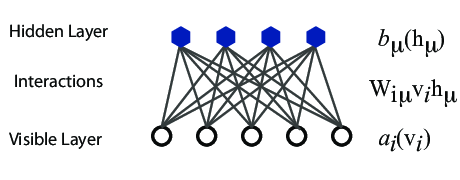
However, they are often hard to train. This leads to the introduction of so-called restricted BMs, or RBMS. Here we take away all lateral connections between nodes in the visible layer as well as connections between nodes in the hidden layer. The network is illustrated in the figure below.
The network layers:
The goal of the hidden layer is to increase the model's expressive power. We encode complex interactions between visible variables by introducing additional, hidden variables that interact with visible degrees of freedom in a simple manner, yet still reproduce the complex correlations between visible degrees in the data once marginalized over (integrated out).
Examples of this trick being employed in physics:
The function \( E(\mathbf{x},\mathbf{h}) \) gives the energy of a configuration (pair of vectors) \( (\mathbf{x}, \mathbf{h}) \). The lower the energy of a configuration, the higher the probability of it. This function also depends on the parameters \( \mathbf{a} \), \( \mathbf{b} \) and \( W \). Thus, when we adjust them during the learning procedure, we are adjusting the energy function to best fit our problem.
An expression for the energy function is $$ E(\hat{x},\hat{h}) = -\sum_{ia}^{NA}b_i^a \alpha_i^a(x_i)-\sum_{jd}^{MD}c_j^d \beta_j^d(h_j)-\sum_{ijad}^{NAMD}b_i^a \alpha_i^a(x_i)c_j^d \beta_j^d(h_j)w_{ij}^{ad}. $$
Here \( \beta_j^d(h_j) \) and \( \alpha_i^a(x_j) \) are so-called transfer functions that map a given input value to a desired feature value. The labels \( a \) and \( d \) denote that there can be multiple transfer functions per variable. The first sum depends only on the visible units. The second on the hidden ones. Note that there is no connection between nodes in a layer.
The quantities \( b \) and \( c \) can be interpreted as the visible and hidden biases, respectively.
The connection between the nodes in the two layers is given by the weights \( w_{ij} \).
RBMs were first developed using binary units in both the visible and hidden layer. The corresponding energy function is defined as follows: $$ \begin{align} E(\mathbf{x}, \mathbf{h}) = - \sum_i^M x_i a_i- \sum_j^N b_j h_j - \sum_{i,j}^{M,N} x_i w_{ij} h_j, \label{_auto5} \end{align} $$ where the binary values taken on by the nodes are most commonly 0 and 1.
Another varient is the RBM where the visible units are Gaussian while the hidden units remain binary: $$ \begin{align} E(\mathbf{x}, \mathbf{h}) = \sum_i^M \frac{(x_i - a_i)^2}{2\sigma_i^2} - \sum_j^N b_j h_j - \sum_{i,j}^{M,N} \frac{x_i w_{ij} h_j}{\sigma_i^2}. \label{_auto6} \end{align} $$
Metropolis sampling starts by suggesting a new configuration \( \boldsymbol{x}^{k+1} \). In the brute force method this is done by some random change of the visible units. The new configuration is then accepted with the acceptance probability $$ \begin{align} A(\boldsymbol{x}^k \rightarrow \boldsymbol{x}^{k+1}) = \text{min} (1, \frac{P(\boldsymbol{x}^{k+1})}{P(\boldsymbol{x}^k)}), \label{_auto7} \end{align} $$ where we need the marginalized probability $$ \begin{align} P(\boldsymbol{x}) &= \sum_\mathbf{h} P_{rbm}(\mathbf{x}, \mathbf{h}) \label{_auto8}\\ &= \frac{1}{Z}\sum_\mathbf{h} e^{-E(\mathbf{x}, \mathbf{h})}. \label{_auto9} \end{align} $$
In this method we sample from the joint probability \( P_{rbm} (\mathbf{x}, \mathbf{h}) \) by way of a two step sampling process. We alternately update the visible and hidden units. New samples are generated according to the conditional probabilities \( P(x_i|\mathbf{h}) \) and \( P(h_j|\mathbf{x}) \) respectively and accepted with the probability of \( 1 \). While the the visible nodes are dependent on the hidden nodes and vice versa, the nodes are independent of other nodes within the same layer. This is due to there being no intra layer interactions in the restricted Boltzmann machine.
The conditional probabilities are often referred to as the activitation functions in the neural networks context due to their role in determining the node outputs. For the binary-binary RBM they are $$ \begin{align} P(h_j = 1 | \boldsymbol{x}) &= \frac{1}{1 + e^{-b_j - \sum_i x_i w_{ij}}} \label{_auto10}\\ P(x_i = 1 | \boldsymbol{h}) &= \frac{1}{1 + e^{-a_j - \sum_j h_j w_{ij}}}, \label{_auto11} \end{align} $$ where we recognize the logistic sigmoid function \( \sigma (x) = 1/(1+exp(-x)) \).
When working with a training dataset, the most common training approach is maximizing the log-likelihood of the training data. The log likelihood characterizes the log-probability of generating the observed data using our generative model. Using this method our cost function is chosen as the negative log-likelihood. The learning then consists of trying to find parameters that maximize the probability of the dataset, and is known as Maximum Likelihood Estimation (MLE). Denoting the parameters as \( \boldsymbol{\theta} = a_1,...,a_M,b_1,...,b_N,w_{11},...,w_{MN} \), the log-likelihood is given by $$ \begin{align} \mathcal{L}(\{ \theta_i \}) &= \langle \text{log} P_\theta(\boldsymbol{x}) \rangle_{data} \label{_auto14}\\ &= - \langle E(\boldsymbol{x}; \{ \theta_i\}) \rangle_{data} - \text{log} Z(\{ \theta_i\}), \label{_auto15} \end{align} $$ where we used that the normalization constant does not depend on the data, \( \langle \text{log} Z(\{ \theta_i\}) \rangle = \text{log} Z(\{ \theta_i\}) \) Our cost function is the negative log-likelihood, \( \mathcal{C}(\{ \theta_i \}) = - \mathcal{L}(\{ \theta_i \}) \)
The training procedure of choice often is Stochastic Gradient Descent (SGD). It consists of a series of iterations where we update the parameters according to the equation $$ \begin{align} \boldsymbol{\theta}_{k+1} = \boldsymbol{\theta}_k - \eta \nabla \mathcal{C} (\boldsymbol{\theta}_k) \label{_auto16} \end{align} $$ at each \( k \)-th iteration. There are a range of variants of the algorithm which aim at making the learning rate \( \eta \) more adaptive so the method might be more efficient while remaining stable.
We now need the gradient of the cost function in order to minimize it. We find that $$ \begin{align} \frac{\partial \mathcal{C}(\{ \theta_i\})}{\partial \theta_i} &= \langle \frac{\partial E(\boldsymbol{x}; \theta_i)}{\partial \theta_i} \rangle_{data} + \frac{\partial \text{log} Z(\{ \theta_i\})}{\partial \theta_i} \label{_auto17}\\ &= \langle O_i(\boldsymbol{x}) \rangle_{data} - \langle O_i(\boldsymbol{x}) \rangle_{model}, \label{_auto18} \end{align} $$ where in order to simplify notation we defined the "operator" $$ \begin{align} O_i(\boldsymbol{x}) = \frac{\partial E(\boldsymbol{x}; \theta_i)}{\partial \theta_i}, \label{_auto19} \end{align} $$ and used the statistical mechanics relationship between expectation values and the log-partition function: $$ \begin{align} \langle O_i(\boldsymbol{x}) \rangle_{model} = \text{Tr} P_\theta(\boldsymbol{x})O_i(\boldsymbol{x}) = - \frac{\partial \text{log} Z(\{ \theta_i\})}{\partial \theta_i}. \label{_auto20} \end{align} $$
The data-dependent term in the gradient is known as the positive phase of the gradient, while the model-dependent term is known as the negative phase of the gradient. The aim of the training is to lower the energy of configurations that are near observed data points (increasing their probability), and raising the energy of configurations that are far from observed data points (decreasing their probability).
The gradient of the negative log-likelihood cost function of a Binary-Binary RBM is then $$ \begin{align} \frac{\partial \mathcal{C} (w_{ij}, a_i, b_j)}{\partial w_{ij}} =& \langle x_i h_j \rangle_{data} - \langle x_i h_j \rangle_{model} \label{_auto21}\\ \frac{\partial \mathcal{C} (w_{ij}, a_i, b_j)}{\partial a_{ij}} =& \langle x_i \rangle_{data} - \langle x_i \rangle_{model} \label{_auto22}\\ \frac{\partial \mathcal{C} (w_{ij}, a_i, b_j)}{\partial b_{ij}} =& \langle h_i \rangle_{data} - \langle h_i \rangle_{model}. \label{_auto23}\\ \label{_auto24} \end{align} $$ To get the expecation values with respect to the data, we set the visible units to each of the observed samples in the training data, then update the hidden units according to the conditional probability found before. We then average over all samples in the training data to calculate expectation values with respect to the data.
To get the expectation values with respect to the model, we use Gibbs sampling. We can either initialize the \( \boldsymbol{x} \) randomly or with a training sample. While we ideally want a large number of Gibbs iterations \( n\rightarrow n \), one might decide to truncate it earlier for efficiency. Doing this while having intialized \( \boldsymbol{x} \) with a training data vector is referred to as contrastive divergence (CD), because one is then closer to approximating the gradient of this function than the negative log-likelihood. The contrastive divergence function is the difference between two Kullback-Leibler divergences (also called relative entropy), which measure how one probability distribution diverges from a second, expected probability distribution (in this case the estimated one from the ground truth one).
When the goal of the training is to approximate a probability distribution, as it is in generative modeling, another relevant measure is the Kullback-Leibler divergence, also known as the relative entropy or Shannon entropy. It is a non-symmetric measure of the dissimilarity between two probability density functions \( p \) and \( q \). If \( p \) is the unkown probability which we approximate with \( q \), we can measure the difference by $$ \begin{align} \text{KL}(p||q) = \int_{-\infty}^{\infty} p (\boldsymbol{x}) \log \frac{p(\boldsymbol{x})}{q(\boldsymbol{x})} d\boldsymbol{x}. \label{_auto25} \end{align} $$
Thus, the Kullback-Leibler divergence between the distribution of the training data \( f(\boldsymbol{x}) \) and the model distribution \( p(\boldsymbol{x}| \boldsymbol{\theta}) \) is $$ \begin{align} \text{KL} (f(\boldsymbol{x})|| p(\boldsymbol{x}| \boldsymbol{\theta})) =& \int_{-\infty}^{\infty} f (\boldsymbol{x}) \log \frac{f(\boldsymbol{x})}{p(\boldsymbol{x}| \boldsymbol{\theta})} d\boldsymbol{x} \label{_auto26}\\ =& \int_{-\infty}^{\infty} f(\boldsymbol{x}) \log f(\boldsymbol{x}) d\boldsymbol{x} - \int_{-\infty}^{\infty} f(\boldsymbol{x}) \log p(\boldsymbol{x}| \boldsymbol{\theta}) d\boldsymbol{x} \label{_auto27}\\ %=& \mathbb{E}_{f(\boldsymbol{x})} (\log f(\boldsymbol{x})) - \mathbb{E}_{f(\boldsymbol{x})} (\log p(\boldsymbol{x}| \boldsymbol{\theta})) =& \langle \log f(\boldsymbol{x}) \rangle_{f(\boldsymbol{x})} - \langle \log p(\boldsymbol{x}| \boldsymbol{\theta}) \rangle_{f(\boldsymbol{x})} \label{_auto28}\\ =& \langle \log f(\boldsymbol{x}) \rangle_{data} + \langle E(\boldsymbol{x}) \rangle_{data} + \log Z \label{_auto29}\\ =& \langle \log f(\boldsymbol{x}) \rangle_{data} + \mathcal{C}_{LL} . \label{_auto30} \end{align} $$
The first term is constant with respect to \( \boldsymbol{\theta} \) since \( f(\boldsymbol{x}) \) is independent of \( \boldsymbol{\theta} \). Thus the Kullback-Leibler Divergence is minimal when the second term is minimal. The second term is the log-likelihood cost function, hence minimizing the Kullback-Leibler divergence is equivalent to maximizing the log-likelihood.
To further understand generative models it is useful to study the gradient of the cost function which is needed in order to minimize it using methods like stochastic gradient descent.
The partition function is the generating function of expectation values, in particular there are mathematical relationships between expectation values and the log-partition function. In this case we have $$ \begin{align} \langle \frac{ \partial E(\boldsymbol{x}; \theta_i) } { \partial \theta_i} \rangle_{model} = \int p(\boldsymbol{x}| \boldsymbol{\theta}) \frac{ \partial E(\boldsymbol{x}; \theta_i) } { \partial \theta_i} d\boldsymbol{x} = -\frac{\partial \log Z(\theta_i)}{ \partial \theta_i} . \label{_auto31} \end{align} $$
Here \( \langle \cdot \rangle_{model} \) is the expectation value over the model probability distribution \( p(\boldsymbol{x}| \boldsymbol{\theta}) \).
Using the previous relationship we can express the gradient of the cost function as $$ \begin{align} \frac{\partial \mathcal{C}_{LL}}{\partial \theta_i} =& \langle \frac{ \partial E(\boldsymbol{x}; \theta_i) } { \partial \theta_i} \rangle_{data} + \frac{\partial \log Z(\theta_i)}{ \partial \theta_i} \label{_auto32}\\ =& \langle \frac{ \partial E(\boldsymbol{x}; \theta_i) } { \partial \theta_i} \rangle_{data} - \langle \frac{ \partial E(\boldsymbol{x}; \theta_i) } { \partial \theta_i} \rangle_{model} \label{_auto33}\\ %=& \langle O_i(\boldsymbol{x}) \rangle_{data} - \langle O_i(\boldsymbol{x}) \rangle_{model} \label{_auto34} \end{align} $$
This expression shows that the gradient of the log-likelihood cost function is a difference of moments, with one calculated from the data and one calculated from the model. The data-dependent term is called the positive phase and the model-dependent term is called the negative phase of the gradient. We see now that minimizing the cost function results in lowering the energy of configurations \( \boldsymbol{x} \) near points in the training data and increasing the energy of configurations not observed in the training data. That means we increase the model's probability of configurations similar to those in the training data.
The gradient of the cost function also demonstrates why gradients of unsupervised, generative models must be computed differently from for those of for example FNNs. While the data-dependent expectation value is easily calculated based on the samples \( \boldsymbol{x}_i \) in the training data, we must sample from the model in order to generate samples from which to caclulate the model-dependent term. We sample from the model by using MCMC-based methods. We can not sample from the model directly because the partition function \( Z \) is generally intractable.
As in supervised machine learning problems, the goal is also here to perform well on unseen data, that is to have good generalization from the training data. The distribution \( f(x) \) we approximate is not the true distribution we wish to estimate, it is limited to the training data. Hence, in unsupervised training as well it is important to prevent overfitting to the training data. Thus it is common to add regularizers to the cost function in the same manner as we discussed for say linear regression.
The idea of applying RBMs to quantum many body problems was presented by G. Carleo and M. Troyer, working with ETH Zurich and Microsoft Research.
Some of their motivation included
Carleo and Troyer applied the RBM to the quantum mechanical spin lattice systems of the Ising model and Heisenberg model, with encouraging results. Our goal is to test the method on systems of moving particles. For the spin lattice systems it was natural to use a binary-binary RBM, with the nodes taking values of 1 and -1. For moving particles, on the other hand, we want the visible nodes to be continuous, representing position coordinates. Thus, we start by choosing a Gaussian-binary RBM, where the visible nodes are continuous and hidden nodes take on values of 0 or 1. If eventually we would like the hidden nodes to be continuous as well the rectified linear units seem like the most relevant choice.
Now this is what we use to represent the wave function, calling it a neural-network quantum state (NQS) $$ \begin{align} \Psi (\mathbf{X}) &= F_{rbm}(\mathbf{x}) \label{_auto38}\\ &= \frac{1}{Z}\sum_{\boldsymbol{h}} e^{-E(\mathbf{x}, \mathbf{h})} \label{_auto39}\\ &= \frac{1}{Z} \sum_{\{h_j\}} e^{-\sum_i^M \frac{(x_i - a_i)^2}{2\sigma^2} + \sum_j^N b_j h_j + \sum_\ {i,j}^{M,N} \frac{x_i w_{ij} h_j}{\sigma^2}} \label{_auto40}\\ &= \frac{1}{Z} e^{-\sum_i^M \frac{(x_i - a_i)^2}{2\sigma^2}} \prod_j^N (1 + e^{b_j + \sum_i^M \frac{x\ _i w_{ij}}{\sigma^2}}). \label{_auto41}\\ \label{_auto42} \end{align} $$
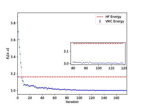
You can find the codes for the simple two-electron case at the Github repository https://github.com/mhjensenseminars/MachineLearningTalk/tree/master/doc/Programs/MLcpp/src. Python codes to come, only c++ as of now.
The trial wave function is based on the product of a Slater determinant with Gaussian orbitals, a simple Jastrow factor \( \exp{(r_{ij})} \) and the reduced Boltzmann machines.
The Broyden-Fletcher-Goldfarb-Shanno algorithm was used to perform the minimization. We used \( 14 \) hidden nodes in the calculations below.