The family of gradient descent methods
Last week we started with linear regression as a case study for the gradient descent methods. Linear regression is a great test case for the gradient descent methods discussed in the lectures since it has several desirable properties such as:
We revisit an example similar to what we had in the first homework set. We have a function of the type
import numpy as np
x = 2*np.random.rand(m,1)
y = 4+3*x+np.random.randn(m,1)
with \( x_i \in [0,1] \) is chosen randomly using a uniform distribution. Additionally we have a stochastic noise chosen according to a normal distribution \( \cal {N}(0,1) \). The linear regression model is given by
$$ h_\theta(x) = \boldsymbol{y} = \theta_0 + \theta_1 x, $$such that
$$ \boldsymbol{y}_i = \theta_0 + \theta_1 x_i. $$Let \( \mathbf{y} = (y_1,\cdots,y_n)^T \), \( \mathbf{\boldsymbol{y}} = (\boldsymbol{y}_1,\cdots,\boldsymbol{y}_n)^T \) and \( \theta = (\theta_0, \theta_1)^T \)
It is convenient to write \( \mathbf{\boldsymbol{y}} = X\theta \) where \( X \in \mathbb{R}^{100 \times 2} \) is the design matrix given by (we keep the intercept here)
$$ X \equiv \begin{bmatrix} 1 & x_1 \\ \vdots & \vdots \\ 1 & x_{100} & \\ \end{bmatrix}. $$The cost/loss/risk function is given by
$$ C(\theta) = \frac{1}{n}||X\theta-\mathbf{y}||_{2}^{2} = \frac{1}{n}\sum_{i=1}^{100}\left[ (\theta_0 + \theta_1 x_i)^2 - 2 y_i (\theta_0 + \theta_1 x_i) + y_i^2\right] $$and we want to find \( \theta \) such that \( C(\theta) \) is minimized.
Computing \( \partial C(\theta) / \partial \theta_0 \) and \( \partial C(\theta) / \partial \theta_1 \) we can show that the gradient can be written as
$$ \nabla_{\theta} C(\theta) = \frac{2}{n}\begin{bmatrix} \sum_{i=1}^{100} \left(\theta_0+\theta_1x_i-y_i\right) \\ \sum_{i=1}^{100}\left( x_i (\theta_0+\theta_1x_i)-y_ix_i\right) \\ \end{bmatrix} = \frac{2}{n}X^T(X\theta - \mathbf{y}), $$where \( X \) is the design matrix defined above.
The Hessian matrix of \( C(\theta) \) is given by
$$ \boldsymbol{H} \equiv \begin{bmatrix} \frac{\partial^2 C(\theta)}{\partial \theta_0^2} & \frac{\partial^2 C(\theta)}{\partial \theta_0 \partial \theta_1} \\ \frac{\partial^2 C(\theta)}{\partial \theta_0 \partial \theta_1} & \frac{\partial^2 C(\theta)}{\partial \theta_1^2} & \\ \end{bmatrix} = \frac{2}{n}X^T X. $$This result implies that \( C(\theta) \) is a convex function since the matrix \( X^T X \) always is positive semi-definite.
We can now write a program that minimizes \( C(\theta) \) using the gradient descent method with a constant learning rate \( \eta \) according to
$$ \theta_{k+1} = \theta_k - \eta \nabla_\theta C(\theta_k), \ k=0,1,\cdots $$We can use the expression we computed for the gradient and let use a \( \theta_0 \) be chosen randomly and let \( \eta = 0.001 \). Stop iterating when \( ||\nabla_\theta C(\theta_k) || \leq \epsilon = 10^{-8} \). Note that the code below does not include the latter stop criterion.
And finally we can compare our solution for \( \theta \) with the analytic result given by \( \theta= (X^TX)^{-1} X^T \mathbf{y} \).
Here our simple example
# Importing various packages
from random import random, seed
import numpy as np
import matplotlib.pyplot as plt
from mpl_toolkits.mplot3d import Axes3D
from matplotlib import cm
from matplotlib.ticker import LinearLocator, FormatStrFormatter
import sys

# the number of datapoints
n = 100
x = 2*np.random.rand(n,1)
y = 4+3*x+np.random.randn(n,1)

X = np.c_[np.ones((n,1)), x]
# Hessian matrix
H = (2.0/n)* X.T @ X
# Get the eigenvalues
EigValues, EigVectors = np.linalg.eig(H)
print(f"Eigenvalues of Hessian Matrix:{EigValues}")

theta_linreg = np.linalg.inv(X.T @ X) @ X.T @ y
print(theta_linreg)
theta = np.random.randn(2,1)

eta = 1.0/np.max(EigValues)
Niterations = 1000

for iter in range(Niterations):
    gradient = (2.0/n)*X.T @ (X @ theta-y)
    theta -= eta*gradient

print(theta)
xnew = np.array([[0],[2]])
xbnew = np.c_[np.ones((2,1)), xnew]
ypredict = xbnew.dot(theta)
ypredict2 = xbnew.dot(theta_linreg)
plt.plot(xnew, ypredict, "r-")
plt.plot(xnew, ypredict2, "b-")
plt.plot(x, y ,'ro')
plt.axis([0,2.0,0, 15.0])
plt.xlabel(r'$x$')
plt.ylabel(r'$y$')
plt.title(r'Gradient descent example')
plt.show()
We have also discussed Ridge regression where the loss function contains a regularized term given by the \( L_2 \) norm of \( \theta \),
$$ C_{\text{ridge}}(\theta) = \frac{1}{n}||X\theta -\mathbf{y}||^2 + \lambda ||\theta||^2, \ \lambda \geq 0. $$In order to minimize \( C_{\text{ridge}}(\theta) \) using GD we adjust the gradient as follows
$$ \nabla_\theta C_{\text{ridge}}(\theta) = \frac{2}{n}\begin{bmatrix} \sum_{i=1}^{100} \left(\theta_0+\theta_1x_i-y_i\right) \\ \sum_{i=1}^{100}\left( x_i (\theta_0+\theta_1x_i)-y_ix_i\right) \\ \end{bmatrix} + 2\lambda\begin{bmatrix} \theta_0 \\ \theta_1\end{bmatrix} = 2 (\frac{1}{n}X^T(X\theta - \mathbf{y})+\lambda \theta). $$We can easily extend our program to minimize \( C_{\text{ridge}}(\theta) \) using gradient descent and compare with the analytical solution given by
$$ \theta_{\text{ridge}} = \left(X^T X + n\lambda I_{2 \times 2} \right)^{-1} X^T \mathbf{y}. $$The Hessian matrix of Ridge Regression for our simple example is given by
$$ \boldsymbol{H} \equiv \begin{bmatrix} \frac{\partial^2 C(\theta)}{\partial \theta_0^2} & \frac{\partial^2 C(\theta)}{\partial \theta_0 \partial \theta_1} \\ \frac{\partial^2 C(\theta)}{\partial \theta_0 \partial \theta_1} & \frac{\partial^2 C(\theta)}{\partial \theta_1^2} & \\ \end{bmatrix} = \frac{2}{n}X^T X+2\lambda\boldsymbol{I}. $$This implies that the Hessian matrix is positive definite, hence the stationary point is a minimum. Note that the Ridge cost function is convex being a sum of two convex functions. Therefore, the stationary point is a global minimum of this function.
from random import random, seed
import numpy as np
import matplotlib.pyplot as plt
from mpl_toolkits.mplot3d import Axes3D
from matplotlib import cm
from matplotlib.ticker import LinearLocator, FormatStrFormatter
import sys

# the number of datapoints
n = 100
x = 2*np.random.rand(n,1)
y = 4+3*x+np.random.randn(n,1)

X = np.c_[np.ones((n,1)), x]
XT_X = X.T @ X

#Ridge parameter lambda
lmbda  = 0.001
Id = n*lmbda* np.eye(XT_X.shape[0])

# Hessian matrix
H = (2.0/n)* XT_X+2*lmbda* np.eye(XT_X.shape[0])
# Get the eigenvalues
EigValues, EigVectors = np.linalg.eig(H)
print(f"Eigenvalues of Hessian Matrix:{EigValues}")


theta_linreg = np.linalg.inv(XT_X+Id) @ X.T @ y
print(theta_linreg)
# Start plain gradient descent
theta = np.random.randn(2,1)

eta = 1.0/np.max(EigValues)
Niterations = 100

for iter in range(Niterations):
    gradients = 2.0/n*X.T @ (X @ (theta)-y)+2*lmbda*theta
    theta -= eta*gradients

print(theta)
ypredict = X @ theta
ypredict2 = X @ theta_linreg
plt.plot(x, ypredict, "r-")
plt.plot(x, ypredict2, "b-")
plt.plot(x, y ,'ro')
plt.axis([0,2.0,0, 15.0])
plt.xlabel(r'$x$')
plt.ylabel(r'$y$')
plt.title(r'Gradient descent example for Ridge')
plt.show()
We discuss here some simple examples where we introduce what is called 'memory'about previous steps, or what is normally called momentum gradient descent. For the mathematical details, see whiteboad notes from lecture on September 8, 2025.
from numpy import asarray
from numpy import arange
from numpy.random import rand
from numpy.random import seed
from matplotlib import pyplot

# objective function
def objective(x):
	return x**2.0

# derivative of objective function
def derivative(x):
	return x * 2.0

# gradient descent algorithm
def gradient_descent(objective, derivative, bounds, n_iter, step_size):
	# track all solutions
	solutions, scores = list(), list()
	# generate an initial point
	solution = bounds[:, 0] + rand(len(bounds)) * (bounds[:, 1] - bounds[:, 0])
	# run the gradient descent
	for i in range(n_iter):
		# calculate gradient
		gradient = derivative(solution)
		# take a step
		solution = solution - step_size * gradient
		# evaluate candidate point
		solution_eval = objective(solution)
		# store solution
		solutions.append(solution)
		scores.append(solution_eval)
		# report progress
		print('>%d f(%s) = %.5f' % (i, solution, solution_eval))
	return [solutions, scores]

# seed the pseudo random number generator
seed(4)
# define range for input
bounds = asarray([[-1.0, 1.0]])
# define the total iterations
n_iter = 30
# define the step size
step_size = 0.1
# perform the gradient descent search
solutions, scores = gradient_descent(objective, derivative, bounds, n_iter, step_size)
# sample input range uniformly at 0.1 increments
inputs = arange(bounds[0,0], bounds[0,1]+0.1, 0.1)
# compute targets
results = objective(inputs)
# create a line plot of input vs result
pyplot.plot(inputs, results)
# plot the solutions found
pyplot.plot(solutions, scores, '.-', color='red')
# show the plot
pyplot.show()
from numpy import asarray
from numpy import arange
from numpy.random import rand
from numpy.random import seed
from matplotlib import pyplot

# objective function
def objective(x):
	return x**2.0

# derivative of objective function
def derivative(x):
	return x * 2.0

# gradient descent algorithm
def gradient_descent(objective, derivative, bounds, n_iter, step_size, momentum):
	# track all solutions
	solutions, scores = list(), list()
	# generate an initial point
	solution = bounds[:, 0] + rand(len(bounds)) * (bounds[:, 1] - bounds[:, 0])
	# keep track of the change
	change = 0.0
	# run the gradient descent
	for i in range(n_iter):
		# calculate gradient
		gradient = derivative(solution)
		# calculate update
		new_change = step_size * gradient + momentum * change
		# take a step
		solution = solution - new_change
		# save the change
		change = new_change
		# evaluate candidate point
		solution_eval = objective(solution)
		# store solution
		solutions.append(solution)
		scores.append(solution_eval)
		# report progress
		print('>%d f(%s) = %.5f' % (i, solution, solution_eval))
	return [solutions, scores]

# seed the pseudo random number generator
seed(4)
# define range for input
bounds = asarray([[-1.0, 1.0]])
# define the total iterations
n_iter = 30
# define the step size
step_size = 0.1
# define momentum
momentum = 0.3
# perform the gradient descent search with momentum
solutions, scores = gradient_descent(objective, derivative, bounds, n_iter, step_size, momentum)
# sample input range uniformly at 0.1 increments
inputs = arange(bounds[0,0], bounds[0,1]+0.1, 0.1)
# compute targets
results = objective(inputs)
# create a line plot of input vs result
pyplot.plot(inputs, results)
# plot the solutions found
pyplot.plot(solutions, scores, '.-', color='red')
# show the plot
pyplot.show()
There are several reasons for using stochastic gradient descent. Some of these are:
In gradient descent we compute the cost function and its gradient for all data points we have.
In large-scale applications such as the ILSVRC challenge, the training data can have on order of millions of examples. Hence, it seems wasteful to compute the full cost function over the entire training set in order to perform only a single parameter update. A very common approach to addressing this challenge is to compute the gradient over batches of the training data. For example, a typical batch could contain some thousand examples from an entire training set of several millions. This batch is then used to perform a parameter update.
In general, stochastic Gradient Descent is Less accurate than gradient descent, as it calculates the gradient on single examples, which may not accurately represent the overall dataset. Gradient Descent is more accurate because it uses the average gradient calculated over the entire dataset.
There are other disadvantages to using SGD. The main drawback is that its convergence behaviour can be more erratic due to the random sampling of individual training examples. This can lead to less accurate results, as the algorithm may not converge to the true minimum of the cost function. Additionally, the learning rate, which determines the step size of each update to the model’s parameters, must be carefully chosen to ensure convergence.
It is however the method of choice in deep learning algorithms where SGD is often used in combination with other optimization techniques, such as momentum or adaptive learning rates
In stochastic gradient descent, the extreme case is the case where we have only one batch, that is we include the whole data set.
This process is called Stochastic Gradient Descent (SGD) (or also sometimes on-line gradient descent). This is relatively less common to see because in practice due to vectorized code optimizations it can be computationally much more efficient to evaluate the gradient for 100 examples, than the gradient for one example 100 times. Even though SGD technically refers to using a single example at a time to evaluate the gradient, you will hear people use the term SGD even when referring to mini-batch gradient descent (i.e. mentions of MGD for “Minibatch Gradient Descent”, or BGD for “Batch gradient descent” are rare to see), where it is usually assumed that mini-batches are used. The size of the mini-batch is a hyperparameter but it is not very common to cross-validate or bootstrap it. It is usually based on memory constraints (if any), or set to some value, e.g. 32, 64 or 128. We use powers of 2 in practice because many vectorized operation implementations work faster when their inputs are sized in powers of 2.
In our notes with SGD we mean stochastic gradient descent with mini-batches.
Stochastic gradient descent (SGD) and variants thereof address some of the shortcomings of the Gradient descent method discussed above.
The underlying idea of SGD comes from the observation that the cost function, which we want to minimize, can almost always be written as a sum over \( n \) data points \( \{\mathbf{x}_i\}_{i=1}^n \),
$$ C(\mathbf{\theta}) = \sum_{i=1}^n c_i(\mathbf{x}_i, \mathbf{\theta}). $$This in turn means that the gradient can be computed as a sum over \( i \)-gradients
$$ \nabla_\theta C(\mathbf{\theta}) = \sum_i^n \nabla_\theta c_i(\mathbf{x}_i, \mathbf{\theta}). $$Stochasticity/randomness is introduced by only taking the gradient on a subset of the data called minibatches. If there are \( n \) data points and the size of each minibatch is \( M \), there will be \( n/M \) minibatches. We denote these minibatches by \( B_k \) where \( k=1,\cdots,n/M \).
As an example, suppose we have \( 10 \) data points \( (\mathbf{x}_1,\cdots, \mathbf{x}_{10}) \) and we choose to have \( M=5 \) minibathces, then each minibatch contains two data points. In particular we have \( B_1 = (\mathbf{x}_1,\mathbf{x}_2), \cdots, B_5 = (\mathbf{x}_9,\mathbf{x}_{10}) \). Note that if you choose \( M=1 \) you have only a single batch with all data points and on the other extreme, you may choose \( M=n \) resulting in a minibatch for each datapoint, i.e \( B_k = \mathbf{x}_k \).
The idea is now to approximate the gradient by replacing the sum over all data points with a sum over the data points in one the minibatches picked at random in each gradient descent step
$$ \nabla_{\theta} C(\mathbf{\theta}) = \sum_{i=1}^n \nabla_\theta c_i(\mathbf{x}_i, \mathbf{\theta}) \rightarrow \sum_{i \in B_k}^n \nabla_\theta c_i(\mathbf{x}_i, \mathbf{\theta}). $$Thus a gradient descent step now looks like
$$ \theta_{j+1} = \theta_j - \eta_j \sum_{i \in B_k}^n \nabla_\theta c_i(\mathbf{x}_i, \mathbf{\theta}) $$where \( k \) is picked at random with equal probability from \( [1,n/M] \). An iteration over the number of minibathces (n/M) is commonly referred to as an epoch. Thus it is typical to choose a number of epochs and for each epoch iterate over the number of minibatches, as exemplified in the code below.
import numpy as np

n = 100 #100 datapoints
M = 5   #size of each minibatch
m = int(n/M) #number of minibatches
n_epochs = 10 #number of epochs

j = 0
for epoch in range(1,n_epochs+1):
    for i in range(m):
        k = np.random.randint(m) #Pick the k-th minibatch at random
        #Compute the gradient using the data in minibatch Bk
        #Compute new suggestion for
        j += 1
Taking the gradient only on a subset of the data has two important benefits. First, it introduces randomness which decreases the chance that our opmization scheme gets stuck in a local minima. Second, if the size of the minibatches are small relative to the number of datapoints (\( M < n \)), the computation of the gradient is much cheaper since we sum over the datapoints in the \( k-th \) minibatch and not all \( n \) datapoints.
A natural question is when do we stop the search for a new minimum? One possibility is to compute the full gradient after a given number of epochs and check if the norm of the gradient is smaller than some threshold and stop if true. However, the condition that the gradient is zero is valid also for local minima, so this would only tell us that we are close to a local/global minimum. However, we could also evaluate the cost function at this point, store the result and continue the search. If the test kicks in at a later stage we can compare the values of the cost function and keep the \( \theta \) that gave the lowest value.
Another approach is to let the step length \( \eta_j \) depend on the number of epochs in such a way that it becomes very small after a reasonable time such that we do not move at all. Such approaches are also called scaling. There are many such ways to scale the learning rate and discussions here. See also https://towardsdatascience.com/learning-rate-schedules-and-adaptive-learning-rate-methods-for-deep-learning-2c8f433990d1 for a discussion of different scaling functions for the learning rate.
As an example, let \( e = 0,1,2,3,\cdots \) denote the current epoch and let \( t_0, t_1 > 0 \) be two fixed numbers. Furthermore, let \( t = e \cdot m + i \) where \( m \) is the number of minibatches and \( i=0,\cdots,m-1 \). Then the function $$\eta_j(t; t_0, t_1) = \frac{t_0}{t+t_1} $$ goes to zero as the number of epochs gets large. I.e. we start with a step length \( \eta_j (0; t_0, t_1) = t_0/t_1 \) which decays in time \( t \).
In this way we can fix the number of epochs, compute \( \theta \) and evaluate the cost function at the end. Repeating the computation will give a different result since the scheme is random by design. Then we pick the final \( \theta \) that gives the lowest value of the cost function.
import numpy as np

def step_length(t,t0,t1):
    return t0/(t+t1)

n = 100 #100 datapoints
M = 5   #size of each minibatch
m = int(n/M) #number of minibatches
n_epochs = 500 #number of epochs
t0 = 1.0
t1 = 10

eta_j = t0/t1
j = 0
for epoch in range(1,n_epochs+1):
    for i in range(m):
        k = np.random.randint(m) #Pick the k-th minibatch at random
        #Compute the gradient using the data in minibatch Bk
        #Compute new suggestion for theta
        t = epoch*m+i
        eta_j = step_length(t,t0,t1)
        j += 1

print("eta_j after %d epochs: %g" % (n_epochs,eta_j))
In the code here we vary the number of mini-batches.
# Importing various packages
from math import exp, sqrt
from random import random, seed
import numpy as np
import matplotlib.pyplot as plt

n = 100
x = 2*np.random.rand(n,1)
y = 4+3*x+np.random.randn(n,1)

X = np.c_[np.ones((n,1)), x]
XT_X = X.T @ X
theta_linreg = np.linalg.inv(X.T @ X) @ (X.T @ y)
print("Own inversion")
print(theta_linreg)
# Hessian matrix
H = (2.0/n)* XT_X
EigValues, EigVectors = np.linalg.eig(H)
print(f"Eigenvalues of Hessian Matrix:{EigValues}")

theta = np.random.randn(2,1)
eta = 1.0/np.max(EigValues)
Niterations = 1000


for iter in range(Niterations):
    gradients = 2.0/n*X.T @ ((X @ theta)-y)
    theta -= eta*gradients
print("theta from own gd")
print(theta)

xnew = np.array([[0],[2]])
Xnew = np.c_[np.ones((2,1)), xnew]
ypredict = Xnew.dot(theta)
ypredict2 = Xnew.dot(theta_linreg)

n_epochs = 50
M = 5   #size of each minibatch
m = int(n/M) #number of minibatches
t0, t1 = 5, 50

def learning_schedule(t):
    return t0/(t+t1)

theta = np.random.randn(2,1)

for epoch in range(n_epochs):
# Can you figure out a better way of setting up the contributions to each batch?
    for i in range(m):
        random_index = M*np.random.randint(m)
        xi = X[random_index:random_index+M]
        yi = y[random_index:random_index+M]
        gradients = (2.0/M)* xi.T @ ((xi @ theta)-yi)
        eta = learning_schedule(epoch*m+i)
        theta = theta - eta*gradients
print("theta from own sdg")
print(theta)

plt.plot(xnew, ypredict, "r-")
plt.plot(xnew, ypredict2, "b-")
plt.plot(x, y ,'ro')
plt.axis([0,2.0,0, 15.0])
plt.xlabel(r'$x$')
plt.ylabel(r'$y$')
plt.title(r'Random numbers ')
plt.show()
In the above code, we have use replacement in setting up the mini-batches. The discussion here may be useful.
Consider minimizing an empirical cost function
$$ C(\theta) =\frac{1}{N}\sum_{i=1}^N l_i(\theta), $$where each \( l_i(\theta) \) is a differentiable loss term. Gradient Descent (GD) updates parameters using the full gradient \( \nabla C(\theta) \), while Stochastic Gradient Descent (SGD) uses a single sample (or mini-batch) gradient \( \nabla l_i(\theta) \) selected at random. In equation form, one GD step is:
$$ \theta_{t+1} = \theta_t-\eta \nabla C(\theta_t) =\theta_t -\eta \frac{1}{N}\sum_{i=1}^N \nabla l_i(\theta_t), $$whereas one SGD step is:
$$ \theta_{t+1} = \theta_t -\eta \nabla l_{i_t}(\theta_t), $$with \( i_t \) randomly chosen. On smooth convex problems, GD and SGD both converge to the global minimum, but their rates differ. GD can take larger, more stable steps since it uses the exact gradient, achieving an error that decreases on the order of \( O(1/t) \) per iteration for convex objectives (and even exponentially fast for strongly convex cases). In contrast, plain SGD has more variance in each step, leading to sublinear convergence in expectation – typically \( O(1/\sqrt{t}) \) for general convex objectives (\thetaith appropriate diminishing step sizes) . Intuitively, GD’s trajectory is smoother and more predictable, while SGD’s path oscillates due to noise but costs far less per iteration, enabling many more updates in the same time.
If \( C(\theta) \) is strongly convex and \( L \)-smooth (so GD enjoys linear convergence), the gap \( C(\theta_t)-C(\theta^*) \) for GD shrinks as
$$ C(\theta_t) - C(\theta^* ) \le \Big(1 - \frac{\mu}{L}\Big)^t [C(\theta_0)-C(\theta^*)], $$a geometric (linear) convergence per iteration . Achieving an \( \epsilon \)-accurate solution thus takes on the order of \( \log(1/\epsilon) \) iterations for GD. However, each GD iteration costs \( O(N) \) gradient evaluations. SGD cannot exploit strong convexity to obtain a linear rate – instead, with a properly decaying step size (e.g. \( \eta_t = \frac{1}{\mu t} \)) or iterate averaging, SGD attains an \( O(1/t) \) convergence rate in expectation . For example, one result of Moulines and Bach 2011, see https://papers.nips.cc/paper_files/paper/2011/hash/40008b9a5380fcacce3976bf7c08af5b-Abstract.html shows that with \( \eta_t = \Theta(1/t) \),
$$ \mathbb{E}[C(\theta_t) - C(\theta^*)] = O(1/t), $$for strongly convex, smooth \( F \) . This \( 1/t \) rate is slower per iteration than GD’s exponential decay, but each SGD iteration is \( N \) times cheaper. In fact, to reach error \( \epsilon \), plain SGD needs on the order of \( T=O(1/\epsilon) \) iterations (sub-linear convergence), while GD needs \( O(\log(1/\epsilon)) \) iterations. When accounting for cost-per-iteration, GD requires \( O(N \log(1/\epsilon)) \) total gradient computations versus SGD’s \( O(1/\epsilon) \) single-sample computations. In large-scale regimes (huge \( N \)), SGD can be faster in wall-clock time because \( N \log(1/\epsilon) \) may far exceed \( 1/\epsilon \) for reasonable accuracy levels. In other words, with millions of data points, one epoch of GD (one full gradient) is extremely costly, whereas SGD can make \( N \) cheap updates in the time GD makes one – often yielding a good solution faster in practice, even though SGD’s asymptotic error decays more slowly. As one lecture succinctly puts it: “SGD can be super effective in terms of iteration cost and memory, but SGD is slow to converge and can’t adapt to strong convexity” . Thus, the break-even point depends on \( N \) and the desired accuracy: for moderate accuracy on very large \( N \), SGD’s cheaper updates win; for extremely high precision (very small \( \epsilon \)) on a modest \( N \), GD’s fast convergence per step can be advantageous.
In non-convex optimization (e.g. deep neural networks), neither GD nor SGD guarantees global minima, but SGD often displays faster progress in finding useful minima. Theoretical results here are weaker, usually showing convergence to a stationary point \( \theta \) (\( |\nabla C| \) is small) in expectation. For example, GD might require \( O(1/\epsilon^2) \) iterations to ensure \( |\nabla C(\theta)| < \epsilon \), and SGD typically has similar polynomial complexity (often worse due to gradient noise). However, a noteworthy difference is that SGD’s stochasticity can help escape saddle points or poor local minima. Random gradient fluctuations act like implicit noise, helping the iterate “jump” out of flat saddle regions where full-batch GD could stagnate . In fact, research has shown that adding noise to GD can guarantee escaping saddle points in polynomial time, and the inherent noise in SGD often serves this role. Empirically, this means SGD can sometimes find a lower loss basin faster, whereas full-batch GD might get “stuck” near saddle points or need a very small learning rate to navigate complex error surfaces . Overall, in modern high-dimensional machine learning, SGD (or mini-batch SGD) is the workhorse for large non-convex problems because it converges to good solutions much faster in practice, despite the lack of a linear convergence guarantee. Full-batch GD is rarely used on large neural networks, as it would require tiny steps to avoid divergence and is extremely slow per iteration .
A major advantage of SGD is its memory efficiency in handling large datasets. Full-batch GD requires access to the entire training set for each iteration, which often means the whole dataset (or a large subset) must reside in memory to compute \( \nabla C(\theta) \) . This results in memory usage that scales linearly with the dataset size \( N \). For instance, if each training sample is large (e.g. high-dimensional features), computing a full gradient may require storing a substantial portion of the data or all intermediate gradients until they are aggregated. In contrast, SGD needs only a single (or a small mini-batch of) training example(s) in memory at any time . The algorithm processes one sample (or mini-batch) at a time and immediately updates the model, discarding that sample before moving to the next. This streaming approach means that memory footprint is essentially independent of \( N \) (apart from storing the model parameters themselves). As one source notes, gradient descent “requires more memory than SGD” because it “must store the entire dataset for each iteration,” whereas SGD “only needs to store the current training example” . In practical terms, if you have a dataset of size, say, 1 million examples, full-batch GD would need memory for all million every step, while SGD could be implemented to load just one example at a time – a crucial benefit if data are too large to fit in RAM or GPU memory. This scalability makes SGD suitable for large-scale learning: as long as you can stream data from disk, SGD can handle arbitrarily large datasets with fixed memory. In fact, SGD “does not need to remember which examples were visited” in the past, allowing it to run in an online fashion on infinite data streams . Full-batch GD, on the other hand, would require multiple passes through a giant dataset per update (or a complex distributed memory system), which is often infeasible.
There is also a secondary memory effect: computing a full-batch gradient in deep learning requires storing all intermediate activations for backpropagation across the entire batch. A very large batch (approaching the full dataset) might exhaust GPU memory due to the need to hold activation gradients for thousands or millions of examples simultaneously. SGD/minibatches mitigate this by splitting the workload – e.g. with a mini-batch of size 32 or 256, memory use stays bounded, whereas a full-batch (size = \( N \)) forward/backward pass could not even be executed if \( N \) is huge. Techniques like gradient accumulation exist to simulate large-batch GD by summing many small-batch gradients – but these still process data in manageable chunks to avoid memory overflow. In summary, memory complexity for GD grows with \( N \), while for SGD it remains \( O(1) \) w.r.t. dataset size (only the model and perhaps a mini-batch reside in memory) . This is a key reason why batch GD “does not scale” to very large data and why virtually all large-scale machine learning algorithms rely on stochastic or mini-batch methods.
Empirical studies strongly support the theoretical trade-offs above. In large-scale machine learning tasks, SGD often converges to a good solution much faster in wall-clock time than full-batch GD, and it uses far less memory. For example, Bottou & Bousquet (2008) analyzed learning time under a fixed computational budget and concluded that when data is abundant, it’s better to use a faster (even if less precise) optimization method to process more examples in the same time . This analysis showed that for large-scale problems, processing more data with SGD yields lower error than spending the time to do exact (batch) optimization on fewer data . In other words, if you have a time budget, it’s often optimal to accept slightly slower convergence per step (as with SGD) in exchange for being able to use many more training samples in that time. This phenomenon is borne out by experiments:
In modern deep learning, full-batch GD is so slow that it is rarely attempted; instead, mini-batch SGD is standard. A recent study demonstrated that it is possible to train a ResNet-50 on ImageNet using full-batch gradient descent, but it required careful tuning (e.g. gradient clipping, tiny learning rates) and vast computational resources – and even then, each full-batch update was extremely expensive.
Using a huge batch (closer to full GD) tends to slow down convergence if the learning rate is not scaled up, and often encounters optimization difficulties (plateaus) that small batches avoid. Empirically, small or medium batch SGD finds minima in fewer clock hours because it can rapidly loop over the data with gradient noise aiding exploration.
From a memory standpoint, practitioners note that batch GD becomes infeasible on large data. For example, if one tried to do full-batch training on a dataset that doesn’t fit in RAM or GPU memory, the program would resort to heavy disk I/O or simply crash. SGD circumvents this by processing mini-batches. Even in cases where data does fit in memory, using a full batch can spike memory usage due to storing all gradients. One empirical observation is that mini-batch training has a “lower, fluctuating usage pattern” of memory, whereas full-batch loading “quickly consumes memory (often exceeding limits)” . This is especially relevant for graph neural networks or other models where a “batch” may include a huge chunk of a graph: full-batch gradient computation can exhaust GPU memory, whereas mini-batch methods keep memory usage manageable .
In summary, SGD converges faster than full-batch GD in terms of actual training time for large-scale problems, provided we measure convergence as reaching a good-enough solution. Theoretical bounds show SGD needs more iterations, but because it performs many more updates per unit time (and requires far less memory), it often achieves lower loss in a given time frame than GD. Full-batch GD might take slightly fewer iterations in theory, but each iteration is so costly that it is “slower… especially for large datasets” . Meanwhile, memory scaling strongly favors SGD: GD’s memory cost grows with dataset size, making it impractical beyond a point, whereas SGD’s memory use is modest and mostly constant w.r.t. \( N \) . These differences have made SGD (and mini-batch variants) the de facto choice for training large machine learning models, from logistic regression on millions of examples to deep neural networks with billions of parameters. The consensus in both research and practice is that for large-scale or high-dimensional tasks, SGD-type methods converge quicker per unit of computation and handle memory constraints better than standard full-batch gradient descent .
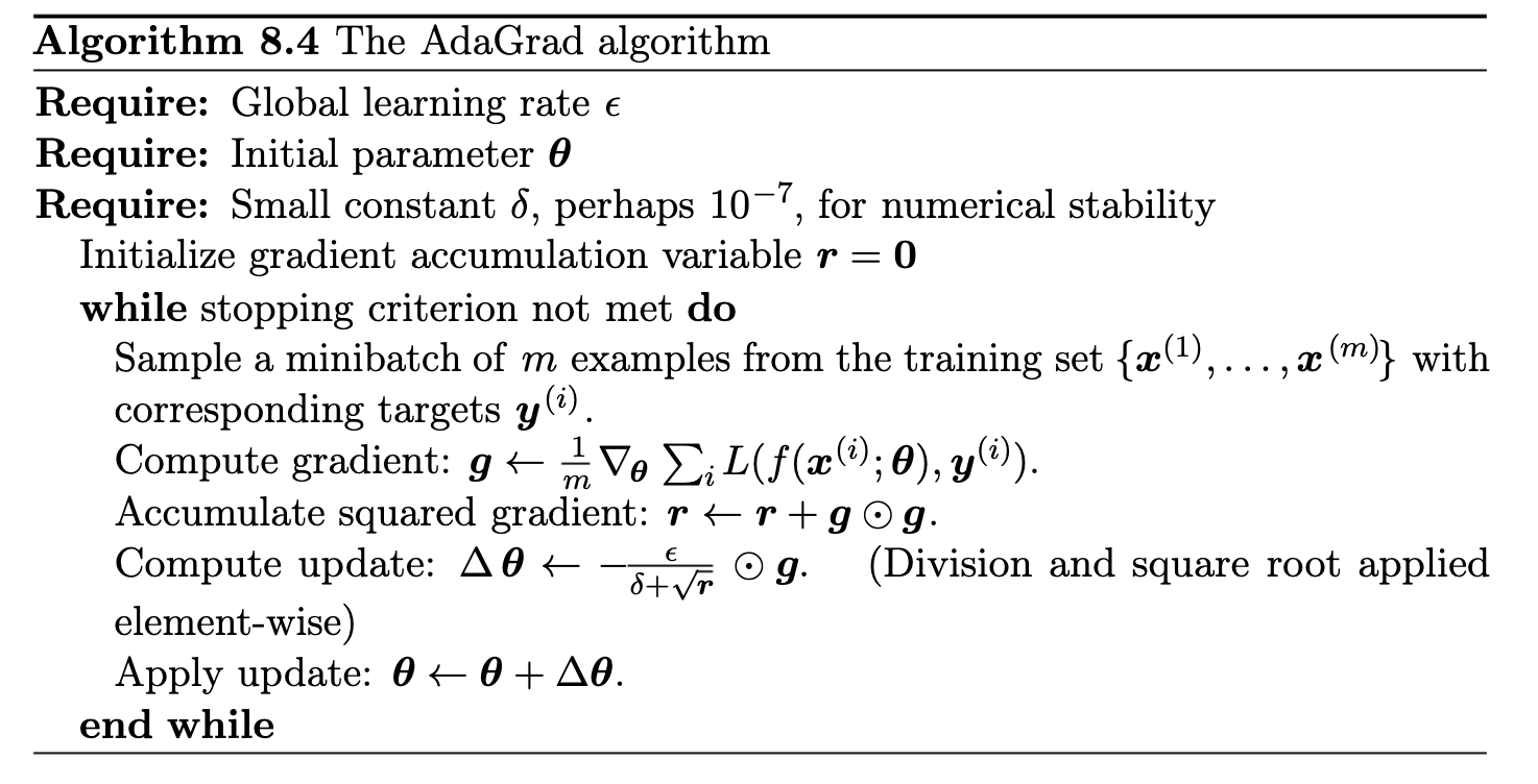
In stochastic gradient descent, with and without momentum, we still have to specify a schedule for tuning the learning rates \( \eta_t \) as a function of time. As discussed in the context of Newton's method, this presents a number of dilemmas. The learning rate is limited by the steepest direction which can change depending on the current position in the landscape. To circumvent this problem, ideally our algorithm would keep track of curvature and take large steps in shallow, flat directions and small steps in steep, narrow directions. Second-order methods accomplish this by calculating or approximating the Hessian and normalizing the learning rate by the curvature. However, this is very computationally expensive for extremely large models. Ideally, we would like to be able to adaptively change the step size to match the landscape without paying the steep computational price of calculating or approximating Hessians.
During the last decade a number of methods have been introduced that accomplish this by tracking not only the gradient, but also the second moment of the gradient. These methods include AdaGrad, AdaDelta, Root Mean Squared Propagation (RMS-Prop), and ADAM.
A fixed \( \eta \) is hard to get right:
In practice, one often uses trial-and-error or schedules (decaying \( \eta \) over time) to find a workable balance. For a function with steep directions and flat directions, a single global \( \eta \) may be inappropriate:
We scale the gradient by the inverse square root of the accumulated matrix \( H_t \). The AdaGrad update at step \( t \) is:
$$ \theta_{t+1} =\theta_t - \eta H_t^{-1/2} g_t, $$where \( H_t^{-1/2} \) is the diagonal matrix with entries \( (r_{t}^{(1)})^{-1/2}, \dots, (r_{t}^{(d)})^{-1/2} \) In coordinates, this means each parameter \( j \) has an individual step size:
$$ \theta_{t+1,j} =\theta_{t,j} -\frac{\eta}{\sqrt{r_{t,j}}}g_{t,j}. $$In practice we add a small constant \( \epsilon \) in the denominator for numerical stability to avoid division by zero:
$$ \theta_{t+1,j}= \theta_{t,j}-\frac{\eta}{\sqrt{\epsilon + r_{t,j}}}g_{t,j}. $$Equivalently, the effective learning rate for parameter \( j \) at time \( t \) is \( \displaystyle \alpha_{t,j} = \frac{\eta}{\sqrt{\epsilon + r_{t,j}}} \). This decreases over time as \( r_{t,j} \) grows.
It effectively reduces the need to tune \( \eta \) by hand.
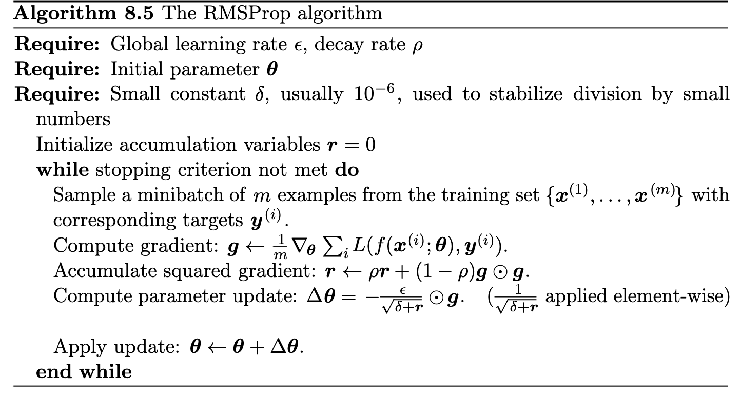
Addresses AdaGrad’s diminishing learning rate issue. Uses a decaying average of squared gradients (instead of a cumulative sum):
$$ v_t = \rho v_{t-1} + (1-\rho)(\nabla C(\theta_t))^2, $$with \( \rho \) typically \( 0.9 \) (or \( 0.99 \)).
RMSProp was first proposed in lecture notes by Geoff Hinton, 2012 – unpublished.)
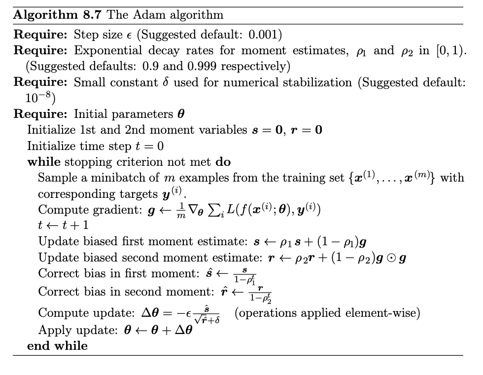
Why combine Momentum and RMSProp? Motivation for Adam: Adaptive Moment Estimation (Adam) was introduced by Kingma an Ba (2014) to combine the benefits of momentum and RMSProp.
Result: Adam is robust, achieves faster convergence with less tuning, and often outperforms SGD (with momentum) in practice.
In ADAM, we keep a running average of both the first and second moment of the gradient and use this information to adaptively change the learning rate for different parameters. The method is efficient when working with large problems involving lots data and/or parameters. It is a combination of the gradient descent with momentum algorithm and the RMSprop algorithm discussed above.
Result: Adam is robust, achieves faster convergence with less tuning, and often outperforms SGD (with momentum) in practice
Adam maintains two moving averages at each time step \( t \) for each parameter \( w \):
The Momentum term
$$ m_t = \beta_1m_{t-1} + (1-\beta_1)\, \nabla C(\theta_t), $$
The RMS term
$$ v_t = \beta_2v_{t-1} + (1-\beta_2)(\nabla C(\theta_t))^2, $$with typical \( \beta_1 = 0.9 \), \( \beta_2 = 0.999 \). Initialize \( m_0 = 0 \), \( v_0 = 0 \).
These are biased estimators of the true first and second moment of the gradients, especially at the start (since \( m_0,v_0 \) are zero)
To counteract initialization bias in \( m_t, v_t \), Adam computes bias-corrected estimates
$$ \hat{m}_t = \frac{m_t}{1 - \beta_1^t}, \qquad \hat{v}_t = \frac{v_t}{1 - \beta_2^t}. $$Finally, Adam updates parameters using the bias-corrected moments:
$$ \theta_{t+1} =\theta_t -\frac{\alpha}{\sqrt{\hat{v}_t} + \epsilon}\hat{m}_t, $$where \( \epsilon \) is a small constant (e.g. \( 10^{-8} \)) to prevent division by zero. Breaking it down:
This is the Adam update rule as given in the original paper.
In practice, Adam often yields faster convergence and better tuning stability than RMSProp or AdaGrad alone
The algorithms we have implemented are well described in the text by Goodfellow, Bengio and Courville, chapter 8.
The codes which implement these algorithms are discussed below here.
In the examples here we take the liberty of sneaking in automatic differentiation (without having discussed the mathematics). In project 1 you will write the gradients as discussed above, that is hard-coding the gradients. By introducing automatic differentiation via the library autograd, which is now replaced by JAX, we have more flexibility in setting up alternative cost functions.
The first example shows results with ordinary leats squares.
# Using Autograd to calculate gradients for OLS
from random import random, seed
import numpy as np
import autograd.numpy as np
import matplotlib.pyplot as plt
from autograd import grad

def CostOLS(theta):
    return (1.0/n)*np.sum((y-X @ theta)**2)

n = 100
x = 2*np.random.rand(n,1)
y = 4+3*x+np.random.randn(n,1)

X = np.c_[np.ones((n,1)), x]
XT_X = X.T @ X
theta_linreg = np.linalg.pinv(XT_X) @ (X.T @ y)
print("Own inversion")
print(theta_linreg)
# Hessian matrix
H = (2.0/n)* XT_X
EigValues, EigVectors = np.linalg.eig(H)
print(f"Eigenvalues of Hessian Matrix:{EigValues}")

theta = np.random.randn(2,1)
eta = 1.0/np.max(EigValues)
Niterations = 1000
# define the gradient
training_gradient = grad(CostOLS)

for iter in range(Niterations):
    gradients = training_gradient(theta)
    theta -= eta*gradients
print("theta from own gd")
print(theta)

xnew = np.array([[0],[2]])
Xnew = np.c_[np.ones((2,1)), xnew]
ypredict = Xnew.dot(theta)
ypredict2 = Xnew.dot(theta_linreg)

plt.plot(xnew, ypredict, "r-")
plt.plot(xnew, ypredict2, "b-")
plt.plot(x, y ,'ro')
plt.axis([0,2.0,0, 15.0])
plt.xlabel(r'$x$')
plt.ylabel(r'$y$')
plt.title(r'Random numbers ')
plt.show()
# Using Autograd to calculate gradients for OLS
from random import random, seed
import numpy as np
import autograd.numpy as np
import matplotlib.pyplot as plt
from autograd import grad

def CostOLS(theta):
    return (1.0/n)*np.sum((y-X @ theta)**2)

n = 100
x = 2*np.random.rand(n,1)
y = 4+3*x#+np.random.randn(n,1)

X = np.c_[np.ones((n,1)), x]
XT_X = X.T @ X
theta_linreg = np.linalg.pinv(XT_X) @ (X.T @ y)
print("Own inversion")
print(theta_linreg)
# Hessian matrix
H = (2.0/n)* XT_X
EigValues, EigVectors = np.linalg.eig(H)
print(f"Eigenvalues of Hessian Matrix:{EigValues}")

theta = np.random.randn(2,1)
eta = 1.0/np.max(EigValues)
Niterations = 30

# define the gradient
training_gradient = grad(CostOLS)

for iter in range(Niterations):
    gradients = training_gradient(theta)
    theta -= eta*gradients
    print(iter,gradients[0],gradients[1])
print("theta from own gd")
print(theta)

# Now improve with momentum gradient descent
change = 0.0
delta_momentum = 0.3
for iter in range(Niterations):
    # calculate gradient
    gradients = training_gradient(theta)
    # calculate update
    new_change = eta*gradients+delta_momentum*change
    # take a step
    theta -= new_change
    # save the change
    change = new_change
    print(iter,gradients[0],gradients[1])
print("theta from own gd wth momentum")
print(theta)
In this code we include the stochastic gradient descent approach discussed above. Note here that we specify which argument we are taking the derivative with respect to when using autograd.
# Using Autograd to calculate gradients using SGD
# OLS example
from random import random, seed
import numpy as np
import autograd.numpy as np
import matplotlib.pyplot as plt
from autograd import grad

# Note change from previous example
def CostOLS(y,X,theta):
    return np.sum((y-X @ theta)**2)

n = 100
x = 2*np.random.rand(n,1)
y = 4+3*x+np.random.randn(n,1)

X = np.c_[np.ones((n,1)), x]
XT_X = X.T @ X
theta_linreg = np.linalg.pinv(XT_X) @ (X.T @ y)
print("Own inversion")
print(theta_linreg)
# Hessian matrix
H = (2.0/n)* XT_X
EigValues, EigVectors = np.linalg.eig(H)
print(f"Eigenvalues of Hessian Matrix:{EigValues}")

theta = np.random.randn(2,1)
eta = 1.0/np.max(EigValues)
Niterations = 1000

# Note that we request the derivative wrt third argument (theta, 2 here)
training_gradient = grad(CostOLS,2)

for iter in range(Niterations):
    gradients = (1.0/n)*training_gradient(y, X, theta)
    theta -= eta*gradients
print("theta from own gd")
print(theta)

xnew = np.array([[0],[2]])
Xnew = np.c_[np.ones((2,1)), xnew]
ypredict = Xnew.dot(theta)
ypredict2 = Xnew.dot(theta_linreg)

plt.plot(xnew, ypredict, "r-")
plt.plot(xnew, ypredict2, "b-")
plt.plot(x, y ,'ro')
plt.axis([0,2.0,0, 15.0])
plt.xlabel(r'$x$')
plt.ylabel(r'$y$')
plt.title(r'Random numbers ')
plt.show()

n_epochs = 50
M = 5   #size of each minibatch
m = int(n/M) #number of minibatches
t0, t1 = 5, 50
def learning_schedule(t):
    return t0/(t+t1)

theta = np.random.randn(2,1)

for epoch in range(n_epochs):
# Can you figure out a better way of setting up the contributions to each batch?
    for i in range(m):
        random_index = M*np.random.randint(m)
        xi = X[random_index:random_index+M]
        yi = y[random_index:random_index+M]
        gradients = (1.0/M)*training_gradient(yi, xi, theta)
        eta = learning_schedule(epoch*m+i)
        theta = theta - eta*gradients
print("theta from own sdg")
print(theta)
# Using Autograd to calculate gradients using SGD
# OLS example
from random import random, seed
import numpy as np
import autograd.numpy as np
import matplotlib.pyplot as plt
from autograd import grad

# Note change from previous example
def CostOLS(y,X,theta):
    return np.sum((y-X @ theta)**2)

n = 100
x = 2*np.random.rand(n,1)
y = 4+3*x+np.random.randn(n,1)

X = np.c_[np.ones((n,1)), x]
XT_X = X.T @ X
theta_linreg = np.linalg.pinv(XT_X) @ (X.T @ y)
print("Own inversion")
print(theta_linreg)
# Hessian matrix
H = (2.0/n)* XT_X
EigValues, EigVectors = np.linalg.eig(H)
print(f"Eigenvalues of Hessian Matrix:{EigValues}")

theta = np.random.randn(2,1)
eta = 1.0/np.max(EigValues)
Niterations = 100

# Note that we request the derivative wrt third argument (theta, 2 here)
training_gradient = grad(CostOLS,2)

for iter in range(Niterations):
    gradients = (1.0/n)*training_gradient(y, X, theta)
    theta -= eta*gradients
print("theta from own gd")
print(theta)


n_epochs = 50
M = 5   #size of each minibatch
m = int(n/M) #number of minibatches
t0, t1 = 5, 50
def learning_schedule(t):
    return t0/(t+t1)

theta = np.random.randn(2,1)

change = 0.0
delta_momentum = 0.3

for epoch in range(n_epochs):
    for i in range(m):
        random_index = M*np.random.randint(m)
        xi = X[random_index:random_index+M]
        yi = y[random_index:random_index+M]
        gradients = (1.0/M)*training_gradient(yi, xi, theta)
        eta = learning_schedule(epoch*m+i)
        # calculate update
        new_change = eta*gradients+delta_momentum*change
        # take a step
        theta -= new_change
        # save the change
        change = new_change
print("theta from own sdg with momentum")
print(theta)
Note that we here have introduced automatic differentiation
# Using Newton's method
from random import random, seed
import numpy as np
import autograd.numpy as np
from autograd import grad

def CostOLS(theta):
    return (1.0/n)*np.sum((y-X @ theta)**2)

n = 100
x = 2*np.random.rand(n,1)
y = 4+3*x+5*x*x

X = np.c_[np.ones((n,1)), x, x*x]
XT_X = X.T @ X
theta_linreg = np.linalg.pinv(XT_X) @ (X.T @ y)
print("Own inversion")
print(theta_linreg)
# Hessian matrix
H = (2.0/n)* XT_X
# Note that here the Hessian does not depend on the parameters theta
invH = np.linalg.pinv(H)
theta = np.random.randn(3,1)
Niterations = 5
# define the gradient
training_gradient = grad(CostOLS)

for iter in range(Niterations):
    gradients = training_gradient(theta)
    theta -= invH @ gradients
    print(iter,gradients[0],gradients[1])
print("theta from own Newton code")
print(theta)
# Using Autograd to calculate gradients using AdaGrad and Stochastic Gradient descent
# OLS example
from random import random, seed
import numpy as np
import autograd.numpy as np
import matplotlib.pyplot as plt
from autograd import grad

# Note change from previous example
def CostOLS(y,X,theta):
    return np.sum((y-X @ theta)**2)

n = 1000
x = np.random.rand(n,1)
y = 2.0+3*x +4*x*x

X = np.c_[np.ones((n,1)), x, x*x]
XT_X = X.T @ X
theta_linreg = np.linalg.pinv(XT_X) @ (X.T @ y)
print("Own inversion")
print(theta_linreg)


# Note that we request the derivative wrt third argument (theta, 2 here)
training_gradient = grad(CostOLS,2)
# Define parameters for Stochastic Gradient Descent
n_epochs = 50
M = 5   #size of each minibatch
m = int(n/M) #number of minibatches
# Guess for unknown parameters theta
theta = np.random.randn(3,1)

# Value for learning rate
eta = 0.01
# Including AdaGrad parameter to avoid possible division by zero
delta  = 1e-8
for epoch in range(n_epochs):
    Giter = 0.0
    for i in range(m):
        random_index = M*np.random.randint(m)
        xi = X[random_index:random_index+M]
        yi = y[random_index:random_index+M]
        gradients = (1.0/M)*training_gradient(yi, xi, theta)
        Giter += gradients*gradients
        update = gradients*eta/(delta+np.sqrt(Giter))
        theta -= update
print("theta from own AdaGrad")
print(theta)
Running this code we note an almost perfect agreement with the results from matrix inversion.
# Using Autograd to calculate gradients using RMSprop  and Stochastic Gradient descent
# OLS example
from random import random, seed
import numpy as np
import autograd.numpy as np
import matplotlib.pyplot as plt
from autograd import grad

# Note change from previous example
def CostOLS(y,X,theta):
    return np.sum((y-X @ theta)**2)

n = 1000
x = np.random.rand(n,1)
y = 2.0+3*x +4*x*x# +np.random.randn(n,1)

X = np.c_[np.ones((n,1)), x, x*x]
XT_X = X.T @ X
theta_linreg = np.linalg.pinv(XT_X) @ (X.T @ y)
print("Own inversion")
print(theta_linreg)


# Note that we request the derivative wrt third argument (theta, 2 here)
training_gradient = grad(CostOLS,2)
# Define parameters for Stochastic Gradient Descent
n_epochs = 50
M = 5   #size of each minibatch
m = int(n/M) #number of minibatches
# Guess for unknown parameters theta
theta = np.random.randn(3,1)

# Value for learning rate
eta = 0.01
# Value for parameter rho
rho = 0.99
# Including AdaGrad parameter to avoid possible division by zero
delta  = 1e-8
for epoch in range(n_epochs):
    Giter = 0.0
    for i in range(m):
        random_index = M*np.random.randint(m)
        xi = X[random_index:random_index+M]
        yi = y[random_index:random_index+M]
        gradients = (1.0/M)*training_gradient(yi, xi, theta)
	# Accumulated gradient
	# Scaling with rho the new and the previous results
        Giter = (rho*Giter+(1-rho)*gradients*gradients)
	# Taking the diagonal only and inverting
        update = gradients*eta/(delta+np.sqrt(Giter))
	# Hadamard product
        theta -= update
print("theta from own RMSprop")
print(theta)
# Using Autograd to calculate gradients using RMSprop  and Stochastic Gradient descent
# OLS example
from random import random, seed
import numpy as np
import autograd.numpy as np
import matplotlib.pyplot as plt
from autograd import grad

# Note change from previous example
def CostOLS(y,X,theta):
    return np.sum((y-X @ theta)**2)

n = 1000
x = np.random.rand(n,1)
y = 2.0+3*x +4*x*x# +np.random.randn(n,1)

X = np.c_[np.ones((n,1)), x, x*x]
XT_X = X.T @ X
theta_linreg = np.linalg.pinv(XT_X) @ (X.T @ y)
print("Own inversion")
print(theta_linreg)


# Note that we request the derivative wrt third argument (theta, 2 here)
training_gradient = grad(CostOLS,2)
# Define parameters for Stochastic Gradient Descent
n_epochs = 50
M = 5   #size of each minibatch
m = int(n/M) #number of minibatches
# Guess for unknown parameters theta
theta = np.random.randn(3,1)

# Value for learning rate
eta = 0.01
# Value for parameters theta1 and theta2, see https://arxiv.org/abs/1412.6980
theta1 = 0.9
theta2 = 0.999
# Including AdaGrad parameter to avoid possible division by zero
delta  = 1e-7
iter = 0
for epoch in range(n_epochs):
    first_moment = 0.0
    second_moment = 0.0
    iter += 1
    for i in range(m):
        random_index = M*np.random.randint(m)
        xi = X[random_index:random_index+M]
        yi = y[random_index:random_index+M]
        gradients = (1.0/M)*training_gradient(yi, xi, theta)
        # Computing moments first
        first_moment = theta1*first_moment + (1-theta1)*gradients
        second_moment = theta2*second_moment+(1-theta2)*gradients*gradients
        first_term = first_moment/(1.0-theta1**iter)
        second_term = second_moment/(1.0-theta2**iter)
	# Scaling with rho the new and the previous results
        update = eta*first_term/(np.sqrt(second_term)+delta)
        theta -= update
print("theta from own ADAM")
print(theta)
For more discussions of Ridge regression and calculation of averages, Wessel van Wieringen's article is highly recommended.
Before fitting a regression model, it is good practice to normalize or standardize the features. This ensures all features are on a comparable scale, which is especially important when using regularization. In the exercises this week we will perform standardization, scaling each feature to have mean 0 and standard deviation 1.
Here we compute the mean and standard deviation of each column (feature) in our design/feature matrix \( \boldsymbol{X} \). Then we subtract the mean and divide by the standard deviation for each feature.
In the example here we we will also center the target \( \boldsymbol{y} \) to mean \( 0 \). Centering \( \boldsymbol{y} \) (and each feature) means the model does not require a separate intercept term, the data is shifted such that the intercept is effectively 0 . (In practice, one could include an intercept in the model and not penalize it, but here we simplify by centering.) Choose \( n=100 \) data points and set up $\boldsymbol{x}, \( \boldsymbol{y} \) and the design matrix \( \boldsymbol{X} \).
# Standardize features (zero mean, unit variance for each feature)
X_mean = X.mean(axis=0)
X_std = X.std(axis=0)
X_std[X_std == 0] = 1  # safeguard to avoid division by zero for constant features
X_norm = (X - X_mean) / X_std

# Center the target to zero mean (optional, to simplify intercept handling)
y_mean = ?
y_centered = ?
Do we need to center the values of \( y \)?
After this preprocessing, each column of \( \boldsymbol{X}_{\mathrm{norm}} \) has mean zero and standard deviation \( 1 \) and \( \boldsymbol{y}_{\mathrm{centered}} \) has mean 0. This can make the optimization landscape nicer and ensures the regularization penalty \( \lambda \sum_j \theta_j^2 \) in Ridge regression treats each coefficient fairly (since features are on the same scale).
Scikit-Learn has several functions which allow us to rescale the data, normally resulting in much better results in terms of various accuracy scores. The StandardScaler function in Scikit-Learn ensures that for each feature/predictor we study the mean value is zero and the variance is one (every column in the design/feature matrix). This scaling has the drawback that it does not ensure that we have a particular maximum or minimum in our data set. Another function included in Scikit-Learn is the MinMaxScaler which ensures that all features are exactly between \( 0 \) and \( 1 \). The
The Normalizer scales each data point such that the feature vector has a euclidean length of one. In other words, it projects a data point on the circle (or sphere in the case of higher dimensions) with a radius of 1. This means every data point is scaled by a different number (by the inverse of it’s length). This normalization is often used when only the direction (or angle) of the data matters, not the length of the feature vector.
The RobustScaler works similarly to the StandardScaler in that it ensures statistical properties for each feature that guarantee that they are on the same scale. However, the RobustScaler uses the median and quartiles, instead of mean and variance. This makes the RobustScaler ignore data points that are very different from the rest (like measurement errors). These odd data points are also called outliers, and might often lead to trouble for other scaling techniques.
Many features are often scaled using standardization to improve performance. In Scikit-Learn this is given by the StandardScaler function as discussed above. It is easy however to write your own. Mathematically, this involves subtracting the mean and divide by the standard deviation over the data set, for each feature:
$$ x_j^{(i)} \rightarrow \frac{x_j^{(i)} - \overline{x}_j}{\sigma(x_j)}, $$where \( \overline{x}_j \) and \( \sigma(x_j) \) are the mean and standard deviation, respectively, of the feature \( x_j \). This ensures that each feature has zero mean and unit standard deviation. For data sets where we do not have the standard deviation or don't wish to calculate it, it is then common to simply set it to one.
Keep in mind that when you transform your data set before training a model, the same transformation needs to be done on your eventual new data set before making a prediction. If we translate this into a Python code, it would could be implemented as
"""
#Model training, we compute the mean value of y and X
y_train_mean = np.mean(y_train)
X_train_mean = np.mean(X_train,axis=0)
X_train = X_train - X_train_mean
y_train = y_train - y_train_mean

# The we fit our model with the training data
trained_model = some_model.fit(X_train,y_train)


#Model prediction, we need also to transform our data set used for the prediction.
X_test = X_test - X_train_mean #Use mean from training data
y_pred = trained_model(X_test)
y_pred = y_pred + y_train_mean
"""
Let us try to understand what this may imply mathematically when we subtract the mean values, also known as zero centering. For simplicity, we will focus on ordinary regression, as done in the above example.
The cost/loss function for regression is
$$ C(\theta_0, \theta_1, ... , \theta_{p-1}) = \frac{1}{n}\sum_{i=0}^{n} \left(y_i - \theta_0 - \sum_{j=1}^{p-1} X_{ij}\theta_j\right)^2,. $$Recall also that we use the squared value. This expression can lead to an increased penalty for higher differences between predicted and output/target values.
What we have done is to single out the \( \theta_0 \) term in the definition of the mean squared error (MSE). The design matrix \( X \) does in this case not contain any intercept column. When we take the derivative with respect to \( \theta_0 \), we want the derivative to obey
$$ \frac{\partial C}{\partial \theta_j} = 0, $$for all \( j \). For \( \theta_0 \) we have
$$ \frac{\partial C}{\partial \theta_0} = -\frac{2}{n}\sum_{i=0}^{n-1} \left(y_i - \theta_0 - \sum_{j=1}^{p-1} X_{ij} \theta_j\right). $$Multiplying away the constant \( 2/n \), we obtain
$$ \sum_{i=0}^{n-1} \theta_0 = \sum_{i=0}^{n-1}y_i - \sum_{i=0}^{n-1} \sum_{j=1}^{p-1} X_{ij} \theta_j. $$Let us specialize first to the case where we have only two parameters \( \theta_0 \) and \( \theta_1 \). Our result for \( \theta_0 \) simplifies then to
$$ n\theta_0 = \sum_{i=0}^{n-1}y_i - \sum_{i=0}^{n-1} X_{i1} \theta_1. $$We obtain then
$$ \theta_0 = \frac{1}{n}\sum_{i=0}^{n-1}y_i - \theta_1\frac{1}{n}\sum_{i=0}^{n-1} X_{i1}. $$If we define
$$ \mu_{\boldsymbol{x}_1}=\frac{1}{n}\sum_{i=0}^{n-1} X_{i1}, $$and the mean value of the outputs as
$$ \mu_y=\frac{1}{n}\sum_{i=0}^{n-1}y_i, $$we have
$$ \theta_0 = \mu_y - \theta_1\mu_{\boldsymbol{x}_1}. $$In the general case with more parameters than \( \theta_0 \) and \( \theta_1 \), we have
$$ \theta_0 = \frac{1}{n}\sum_{i=0}^{n-1}y_i - \frac{1}{n}\sum_{i=0}^{n-1}\sum_{j=1}^{p-1} X_{ij}\theta_j. $$We can rewrite the latter equation as
$$ \theta_0 = \frac{1}{n}\sum_{i=0}^{n-1}y_i - \sum_{j=1}^{p-1} \mu_{\boldsymbol{x}_j}\theta_j, $$where we have defined
$$ \mu_{\boldsymbol{x}_j}=\frac{1}{n}\sum_{i=0}^{n-1} X_{ij}, $$the mean value for all elements of the column vector \( \boldsymbol{x}_j \).
Replacing \( y_i \) with \( y_i - y_i - \overline{\boldsymbol{y}} \) and centering also our design matrix results in a cost function (in vector-matrix disguise)
$$ C(\boldsymbol{\theta}) = (\boldsymbol{\tilde{y}} - \tilde{X}\boldsymbol{\theta})^T(\boldsymbol{\tilde{y}} - \tilde{X}\boldsymbol{\theta}). $$If we minimize with respect to \( \boldsymbol{\theta} \) we have then
$$ \hat{\boldsymbol{\theta}} = (\tilde{X}^T\tilde{X})^{-1}\tilde{X}^T\boldsymbol{\tilde{y}}, $$where \( \boldsymbol{\tilde{y}} = \boldsymbol{y} - \overline{\boldsymbol{y}} \) and \( \tilde{X}_{ij} = X_{ij} - \frac{1}{n}\sum_{k=0}^{n-1}X_{kj} \).
For Ridge regression we need to add \( \lambda \boldsymbol{\theta}^T\boldsymbol{\theta} \) to the cost function and get then
$$ \hat{\boldsymbol{\theta}} = (\tilde{X}^T\tilde{X} + \lambda I)^{-1}\tilde{X}^T\boldsymbol{\tilde{y}}. $$What does this mean? And why do we insist on all this? Let us look at some examples.
This code shows a simple first-order fit to a data set using the above transformed data, where we consider the role of the intercept first, by either excluding it or including it (code example thanks to Øyvind Sigmundson Schøyen). Here our scaling of the data is done by subtracting the mean values only. Note also that we do not split the data into training and test.
import numpy as np
import matplotlib.pyplot as plt

from sklearn.linear_model import LinearRegression


np.random.seed(2021)

def MSE(y_data,y_model):
    n = np.size(y_model)
    return np.sum((y_data-y_model)**2)/n


def fit_theta(X, y):
    return np.linalg.pinv(X.T @ X) @ X.T @ y


true_theta = [2, 0.5, 3.7]

x = np.linspace(0, 1, 11)
y = np.sum(
    np.asarray([x ** p * b for p, b in enumerate(true_theta)]), axis=0
) + 0.1 * np.random.normal(size=len(x))

degree = 3
X = np.zeros((len(x), degree))

# Include the intercept in the design matrix
for p in range(degree):
    X[:, p] = x ** p

theta = fit_theta(X, y)

# Intercept is included in the design matrix
skl = LinearRegression(fit_intercept=False).fit(X, y)

print(f"True theta: {true_theta}")
print(f"Fitted theta: {theta}")
print(f"Sklearn fitted theta: {skl.coef_}")
ypredictOwn = X @ theta
ypredictSKL = skl.predict(X)
print(f"MSE with intercept column")
print(MSE(y,ypredictOwn))
print(f"MSE with intercept column from SKL")
print(MSE(y,ypredictSKL))


plt.figure()
plt.scatter(x, y, label="Data")
plt.plot(x, X @ theta, label="Fit")
plt.plot(x, skl.predict(X), label="Sklearn (fit_intercept=False)")


# Do not include the intercept in the design matrix
X = np.zeros((len(x), degree - 1))

for p in range(degree - 1):
    X[:, p] = x ** (p + 1)

# Intercept is not included in the design matrix
skl = LinearRegression(fit_intercept=True).fit(X, y)

# Use centered values for X and y when computing coefficients
y_offset = np.average(y, axis=0)
X_offset = np.average(X, axis=0)

theta = fit_theta(X - X_offset, y - y_offset)
intercept = np.mean(y_offset - X_offset @ theta)

print(f"Manual intercept: {intercept}")
print(f"Fitted theta (without intercept): {theta}")
print(f"Sklearn intercept: {skl.intercept_}")
print(f"Sklearn fitted theta (without intercept): {skl.coef_}")
ypredictOwn = X @ theta
ypredictSKL = skl.predict(X)
print(f"MSE with Manual intercept")
print(MSE(y,ypredictOwn+intercept))
print(f"MSE with Sklearn intercept")
print(MSE(y,ypredictSKL))

plt.plot(x, X @ theta + intercept, "--", label="Fit (manual intercept)")
plt.plot(x, skl.predict(X), "--", label="Sklearn (fit_intercept=True)")
plt.grid()
plt.legend()

plt.show()
The intercept is the value of our output/target variable when all our features are zero and our function crosses the \( y \)-axis (for a one-dimensional case).
Printing the MSE, we see first that both methods give the same MSE, as they should. However, when we move to for example Ridge regression, the way we treat the intercept may give a larger or smaller MSE, meaning that the MSE can be penalized by the value of the intercept. Not including the intercept in the fit, means that the regularization term does not include \( \theta_0 \). For different values of \( \lambda \), this may lead to different MSE values.
To remind the reader, the regularization term, with the intercept in Ridge regression, is given by
$$ \lambda \vert\vert \boldsymbol{\theta} \vert\vert_2^2 = \lambda \sum_{j=0}^{p-1}\theta_j^2, $$but when we take out the intercept, this equation becomes
$$ \lambda \vert\vert \boldsymbol{\theta} \vert\vert_2^2 = \lambda \sum_{j=1}^{p-1}\theta_j^2. $$For Lasso regression we have
$$ \lambda \vert\vert \boldsymbol{\theta} \vert\vert_1 = \lambda \sum_{j=1}^{p-1}\vert\theta_j\vert. $$It means that, when scaling the design matrix and the outputs/targets, by subtracting the mean values, we have an optimization problem which is not penalized by the intercept. The MSE value can then be smaller since it focuses only on the remaining quantities. If we however bring back the intercept, we will get a MSE which then contains the intercept.
Armed with this wisdom, we attempt first to simply set the intercept equal to False in our implementation of Ridge regression for our well-known vanilla data set.
import numpy as np
import pandas as pd
import matplotlib.pyplot as plt
from sklearn.model_selection import train_test_split
from sklearn import linear_model

def MSE(y_data,y_model):
    n = np.size(y_model)
    return np.sum((y_data-y_model)**2)/n


# A seed just to ensure that the random numbers are the same for every run.
# Useful for eventual debugging.
np.random.seed(3155)

n = 100
x = np.random.rand(n)
y = np.exp(-x**2) + 1.5 * np.exp(-(x-2)**2)

Maxpolydegree = 20
X = np.zeros((n,Maxpolydegree))
#We include explicitely the intercept column
for degree in range(Maxpolydegree):
    X[:,degree] = x**degree
# We split the data in test and training data
X_train, X_test, y_train, y_test = train_test_split(X, y, test_size=0.2)

p = Maxpolydegree
I = np.eye(p,p)
# Decide which values of lambda to use
nlambdas = 6
MSEOwnRidgePredict = np.zeros(nlambdas)
MSERidgePredict = np.zeros(nlambdas)
lambdas = np.logspace(-4, 2, nlambdas)
for i in range(nlambdas):
    lmb = lambdas[i]
    OwnRidgeTheta = np.linalg.pinv(X_train.T @ X_train+lmb*I) @ X_train.T @ y_train
    # Note: we include the intercept column and no scaling
    RegRidge = linear_model.Ridge(lmb,fit_intercept=False)
    RegRidge.fit(X_train,y_train)
    # and then make the prediction
    ytildeOwnRidge = X_train @ OwnRidgeTheta
    ypredictOwnRidge = X_test @ OwnRidgeTheta
    ytildeRidge = RegRidge.predict(X_train)
    ypredictRidge = RegRidge.predict(X_test)
    MSEOwnRidgePredict[i] = MSE(y_test,ypredictOwnRidge)
    MSERidgePredict[i] = MSE(y_test,ypredictRidge)
    print("Theta values for own Ridge implementation")
    print(OwnRidgeTheta)
    print("Theta values for Scikit-Learn Ridge implementation")
    print(RegRidge.coef_)
    print("MSE values for own Ridge implementation")
    print(MSEOwnRidgePredict[i])
    print("MSE values for Scikit-Learn Ridge implementation")
    print(MSERidgePredict[i])

# Now plot the results
plt.figure()
plt.plot(np.log10(lambdas), MSEOwnRidgePredict, 'r', label = 'MSE own Ridge Test')
plt.plot(np.log10(lambdas), MSERidgePredict, 'g', label = 'MSE Ridge Test')

plt.xlabel('log10(lambda)')
plt.ylabel('MSE')
plt.legend()
plt.show()
The results here agree when we force Scikit-Learn's Ridge function to include the first column in our design matrix. We see that the results agree very well. Here we have thus explicitely included the intercept column in the design matrix. What happens if we do not include the intercept in our fit? Let us see how we can change this code by zero centering.
import numpy as np
import pandas as pd
import matplotlib.pyplot as plt
from sklearn.model_selection import train_test_split
from sklearn import linear_model
from sklearn.preprocessing import StandardScaler

def MSE(y_data,y_model):
    n = np.size(y_model)
    return np.sum((y_data-y_model)**2)/n
# A seed just to ensure that the random numbers are the same for every run.
# Useful for eventual debugging.
np.random.seed(315)

n = 100
x = np.random.rand(n)
y = np.exp(-x**2) + 1.5 * np.exp(-(x-2)**2)

Maxpolydegree = 20
X = np.zeros((n,Maxpolydegree-1))

for degree in range(1,Maxpolydegree): #No intercept column
    X[:,degree-1] = x**(degree)

# We split the data in test and training data
X_train, X_test, y_train, y_test = train_test_split(X, y, test_size=0.2)

#For our own implementation, we will need to deal with the intercept by centering the design matrix and the target variable
X_train_mean = np.mean(X_train,axis=0)
#Center by removing mean from each feature
X_train_scaled = X_train - X_train_mean
X_test_scaled = X_test - X_train_mean
#The model intercept (called y_scaler) is given by the mean of the target variable (IF X is centered)
#Remove the intercept from the training data.
y_scaler = np.mean(y_train)
y_train_scaled = y_train - y_scaler

p = Maxpolydegree-1
I = np.eye(p,p)
# Decide which values of lambda to use
nlambdas = 6
MSEOwnRidgePredict = np.zeros(nlambdas)
MSERidgePredict = np.zeros(nlambdas)

lambdas = np.logspace(-4, 2, nlambdas)
for i in range(nlambdas):
    lmb = lambdas[i]
    OwnRidgeTheta = np.linalg.pinv(X_train_scaled.T @ X_train_scaled+lmb*I) @ X_train_scaled.T @ (y_train_scaled)
    intercept_ = y_scaler - X_train_mean@OwnRidgeTheta #The intercept can be shifted so the model can predict on uncentered data
    #Add intercept to prediction
    ypredictOwnRidge = X_test_scaled @ OwnRidgeTheta + y_scaler
    RegRidge = linear_model.Ridge(lmb)
    RegRidge.fit(X_train,y_train)
    ypredictRidge = RegRidge.predict(X_test)
    MSEOwnRidgePredict[i] = MSE(y_test,ypredictOwnRidge)
    MSERidgePredict[i] = MSE(y_test,ypredictRidge)
    print("Theta values for own Ridge implementation")
    print(OwnRidgeTheta) #Intercept is given by mean of target variable
    print("Theta values for Scikit-Learn Ridge implementation")
    print(RegRidge.coef_)
    print('Intercept from own implementation:')
    print(intercept_)
    print('Intercept from Scikit-Learn Ridge implementation')
    print(RegRidge.intercept_)
    print("MSE values for own Ridge implementation")
    print(MSEOwnRidgePredict[i])
    print("MSE values for Scikit-Learn Ridge implementation")
    print(MSERidgePredict[i])


# Now plot the results
plt.figure()
plt.plot(np.log10(lambdas), MSEOwnRidgePredict, 'b--', label = 'MSE own Ridge Test')
plt.plot(np.log10(lambdas), MSERidgePredict, 'g--', label = 'MSE SL Ridge Test')
plt.xlabel('log10(lambda)')
plt.ylabel('MSE')
plt.legend()
plt.show()
We see here, when compared to the code which includes explicitely the intercept column, that our MSE value is actually smaller. This is because the regularization term does not include the intercept value \( \theta_0 \) in the fitting. This applies to Lasso regularization as well. It means that our optimization is now done only with the centered matrix and/or vector that enter the fitting procedure.