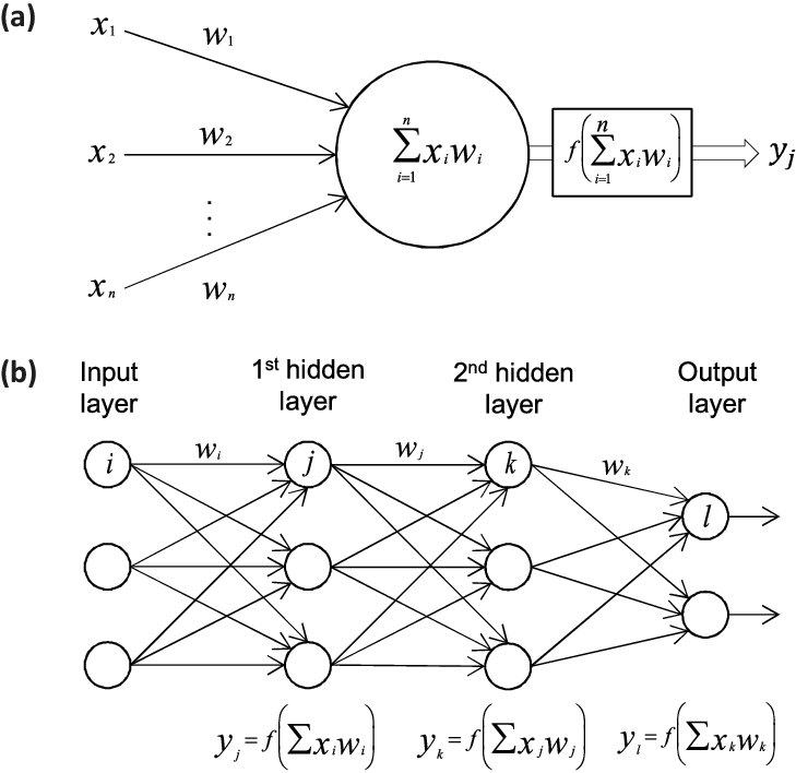
Figure 1: In a) we show a single perceptron model while in b) we dispay a network with two hidden layers, an input layer and an output layer.
Aim: Getting started with coding neural network. The exercises this week aim at setting up the feed-forward part of a neural network.
Artificial neural networks are computational systems that can learn to perform tasks by considering examples, generally without being programmed with any task-specific rules. It is supposed to mimic a biological system, wherein neurons interact by sending signals in the form of mathematical functions between layers. All layers can contain an arbitrary number of neurons, and each connection is represented by a weight variable.
The field of artificial neural networks has a long history of development, and is closely connected with the advancement of computer science and computers in general. A model of artificial neurons was first developed by McCulloch and Pitts in 1943 to study signal processing in the brain and has later been refined by others. The general idea is to mimic neural networks in the human brain, which is composed of billions of neurons that communicate with each other by sending electrical signals. Each neuron accumulates its incoming signals, which must exceed an activation threshold to yield an output. If the threshold is not overcome, the neuron remains inactive, i.e. has zero output.
This behaviour has inspired a simple mathematical model for an artificial neuron.
$$ \begin{equation} y = f\left(\sum_{i=1}^n w_ix_i\right) = f(u) \label{artificialNeuron} \end{equation} $$Here, the output \( y \) of the neuron is the value of its activation function, which have as input a weighted sum of signals \( x_i, \dots ,x_n \) received by \( n \) other neurons.
Conceptually, it is helpful to divide neural networks into four categories:
In natural science, DNNs and CNNs have already found numerous applications. In statistical physics, they have been applied to detect phase transitions in 2D Ising and Potts models, lattice gauge theories, and different phases of polymers, or solving the Navier-Stokes equation in weather forecasting. Deep learning has also found interesting applications in quantum physics. Various quantum phase transitions can be detected and studied using DNNs and CNNs, topological phases, and even non-equilibrium many-body localization. Representing quantum states as DNNs quantum state tomography are among some of the impressive achievements to reveal the potential of DNNs to facilitate the study of quantum systems.
In quantum information theory, it has been shown that one can perform gate decompositions with the help of neural.
The applications are not limited to the natural sciences. There is a plethora of applications in essentially all disciplines, from the humanities to life science and medicine.
An artificial neural network (ANN), is a computational model that consists of layers of connected neurons, or nodes or units. We will refer to these interchangeably as units or nodes, and sometimes as neurons.
It is supposed to mimic a biological nervous system by letting each neuron interact with other neurons by sending signals in the form of mathematical functions between layers. A wide variety of different ANNs have been developed, but most of them consist of an input layer, an output layer and eventual layers in-between, called hidden layers. All layers can contain an arbitrary number of nodes, and each connection between two nodes is associated with a weight variable.
Neural networks (also called neural nets) are neural-inspired nonlinear models for supervised learning. As we will see, neural nets can be viewed as natural, more powerful extensions of supervised learning methods such as linear and logistic regression and soft-max methods we discussed earlier.
The feed-forward neural network (FFNN) was the first and simplest type of ANNs that were devised. In this network, the information moves in only one direction: forward through the layers.
Nodes are represented by circles, while the arrows display the connections between the nodes, including the direction of information flow. Additionally, each arrow corresponds to a weight variable (figure to come). We observe that each node in a layer is connected to all nodes in the subsequent layer, making this a so-called fully-connected FFNN.
A different variant of FFNNs are convolutional neural networks (CNNs), which have a connectivity pattern inspired by the animal visual cortex. Individual neurons in the visual cortex only respond to stimuli from small sub-regions of the visual field, called a receptive field. This makes the neurons well-suited to exploit the strong spatially local correlation present in natural images. The response of each neuron can be approximated mathematically as a convolution operation. (figure to come)
Convolutional neural networks emulate the behaviour of neurons in the visual cortex by enforcing a local connectivity pattern between nodes of adjacent layers: Each node in a convolutional layer is connected only to a subset of the nodes in the previous layer, in contrast to the fully-connected FFNN. Often, CNNs consist of several convolutional layers that learn local features of the input, with a fully-connected layer at the end, which gathers all the local data and produces the outputs. They have wide applications in image and video recognition.
So far we have only mentioned ANNs where information flows in one direction: forward. Recurrent neural networks on the other hand, have connections between nodes that form directed cycles. This creates a form of internal memory which are able to capture information on what has been calculated before; the output is dependent on the previous computations. Recurrent NNs make use of sequential information by performing the same task for every element in a sequence, where each element depends on previous elements. An example of such information is sentences, making recurrent NNs especially well-suited for handwriting and speech recognition.
There are many other kinds of ANNs that have been developed. One type that is specifically designed for interpolation in multidimensional space is the radial basis function (RBF) network. RBFs are typically made up of three layers: an input layer, a hidden layer with non-linear radial symmetric activation functions and a linear output layer (''linear'' here means that each node in the output layer has a linear activation function). The layers are normally fully-connected and there are no cycles, thus RBFs can be viewed as a type of fully-connected FFNN. They are however usually treated as a separate type of NN due the unusual activation functions.
One uses often so-called fully-connected feed-forward neural networks with three or more layers (an input layer, one or more hidden layers and an output layer) consisting of neurons that have non-linear activation functions.
Such networks are often called multilayer perceptrons (MLPs).
According to the Universal approximation theorem, a feed-forward neural network with just a single hidden layer containing a finite number of neurons can approximate a continuous multidimensional function to arbitrary accuracy, assuming the activation function for the hidden layer is a non-constant, bounded and monotonically-increasing continuous function.
Note that the requirements on the activation function only applies to the hidden layer, the output nodes are always assumed to be linear, so as to not restrict the range of output values.
Figure 1: In a) we show a single perceptron model while in b) we dispay a network with two hidden layers, an input layer and an output layer.
Neural networks, in its so-called feed-forward form, where each iterations contains a feed-forward stage and a back-propgagation stage, consist of series of affine matrix-matrix and matrix-vector multiplications. The unknown parameters (the so-called biases and weights which deternine the architecture of a neural network), are uptaded iteratively using the so-called back-propagation algorithm. This algorithm corresponds to the so-called reverse mode of automatic differentation.
A neural network consists of a series of hidden layers, in addition to the input and output layers. Each layer \( l \) has a set of parameters \( \boldsymbol{\Theta}^{(l)}=(\boldsymbol{W}^{(l)},\boldsymbol{b}^{(l)}) \) which are related to the parameters in other layers through a series of affine transformations, for a standard NN these are matrix-matrix and matrix-vector multiplications. For all layers we will simply use a collective variable \( \boldsymbol{\Theta} \).
It consist of two basic steps:
These two steps make up one iteration. This iterative process is continued till we reach an eventual stopping criterion.
The architecture of a neural network defines our model. This model aims at describing some function \( f(\boldsymbol{x} \) which represents some final result (outputs or tagrget values) given a specific inpput \( \boldsymbol{x} \). Note that here \( \boldsymbol{y} \) and \( \boldsymbol{x} \) are not limited to be vectors.
The architecture consists of
The cost function is a function of the unknown parameters \( \boldsymbol{\Theta} \) where the latter is a container for all possible parameters needed to define a neural network
If we are dealing with a regression task a typical cost/loss function is the mean squared error
$$ C(\boldsymbol{\Theta})=\frac{1}{n}\left\{\left(\boldsymbol{y}-\boldsymbol{X}\boldsymbol{\theta}\right)^T\left(\boldsymbol{y}-\boldsymbol{X}\boldsymbol{\theta}\right)\right\}. $$This function represents one of many possible ways to define the so-called cost function. Note that here we have assumed a linear dependence in terms of the paramters \( \boldsymbol{\Theta} \). This is in general not the case.
For neural networks the parameters \( \boldsymbol{\Theta} \) are given by the so-called weights and biases (to be defined below).
The weights are given by matrix elements \( w_{ij}^{(l)} \) where the superscript indicates the layer number. The biases are typically given by vector elements representing each single node of a given layer, that is \( b_j^{(l)} \).
Having defined the architecture of a neural network, the optimization of the cost function with respect to the parameters \( \boldsymbol{\Theta} \), involves the calculations of gradients and their optimization. The gradients represent the derivatives of a multidimensional object and are often approximated by various gradient methods, including
In addition to the above, there are often additional hyperparamaters which are included in the setup of a neural network. These will be discussed below.
The universal approximation theorem plays a central role in deep learning. Cybenko (1989) showed the following:
Let \( \sigma \) be any continuous sigmoidal function such that
$$ \sigma(z) = \left\{\begin{array}{cc} 1 & z\rightarrow \infty\\ 0 & z \rightarrow -\infty \end{array}\right. $$Given a continuous and deterministic function \( F(\boldsymbol{x}) \) on the unit cube in \( d \)-dimensions \( F\in [0,1]^d \), \( x\in [0,1]^d \) and a parameter \( \epsilon >0 \), there is a one-layer (hidden) neural network \( f(\boldsymbol{x};\boldsymbol{\Theta}) \) with \( \boldsymbol{\Theta}=(\boldsymbol{W},\boldsymbol{b}) \) and \( \boldsymbol{W}\in \mathbb{R}^{m\times n} \) and \( \boldsymbol{b}\in \mathbb{R}^{n} \), for which
$$ \vert F(\boldsymbol{x})-f(\boldsymbol{x};\boldsymbol{\Theta})\vert < \epsilon \hspace{0.1cm} \forall \boldsymbol{x}\in[0,1]^d. $$For those of you familiar with for example the Stone-Weierstrass theorem for polynomial approximations or the convergence criterion for Fourier series, there are similarities in the derivation of the proof for neural networks.
Any continuous function \( y=F(\boldsymbol{x}) \) supported on the unit cube in \( d \)-dimensions can be approximated by a one-layer sigmoidal network to arbitrary accuracy.
Hornik (1991) extended the theorem by letting any non-constant, bounded activation function to be included using that the expectation value
$$ \mathbb{E}[\vert F(\boldsymbol{x})\vert^2] =\int_{\boldsymbol{x}\in D} \vert F(\boldsymbol{x})\vert^2p(\boldsymbol{x})d\boldsymbol{x} < \infty. $$Then we have
$$ \mathbb{E}[\vert F(\boldsymbol{x})-f(\boldsymbol{x};\boldsymbol{\Theta})\vert^2] =\int_{\boldsymbol{x}\in D} \vert F(\boldsymbol{x})-f(\boldsymbol{x};\boldsymbol{\Theta})\vert^2p(\boldsymbol{x})d\boldsymbol{x} < \epsilon. $$None of the proofs give any insight into the relation between the number of of hidden layers and nodes and the approximation error \( \epsilon \), nor the magnitudes of \( \boldsymbol{W} \) and \( \boldsymbol{b} \).
Neural networks (NNs) have what we may call a kind of universality no matter what function we want to compute.
It does not mean that an NN can be used to exactly compute any function. Rather, we get an approximation that is as good as we want.
The class of functions that can be approximated are the continuous ones. If the function \( F(\boldsymbol{x}) \) is discontinuous, it won't in general be possible to approximate it. However, an NN may still give an approximation even if we fail in some points.
The questions we want to ask are how do changes in the biases and the weights in our network change the cost function and how can we use the final output to modify the weights and biases?
To derive these equations let us start with a plain regression problem and define our cost function as
$$ {\cal C}(\boldsymbol{\Theta}) = \frac{1}{2}\sum_{i=1}^n\left(y_i - \tilde{y}_i\right)^2, $$where the $y_i$s are our \( n \) targets (the values we want to reproduce), while the outputs of the network after having propagated all inputs \( \boldsymbol{x} \) are given by \( \boldsymbol{\tilde{y}}_i \).

With our definition of the targets \( \boldsymbol{y} \), the outputs of the network \( \boldsymbol{\tilde{y}} \) and the inputs \( \boldsymbol{x} \) we define now the activation \( z_j^l \) of node/neuron/unit \( j \) of the \( l \)-th layer as a function of the bias, the weights which add up from the previous layer \( l-1 \) and the forward passes/outputs \( \hat{a}^{l-1} \) from the previous layer as
$$ z_j^l = \sum_{i=1}^{M_{l-1}}w_{ij}^la_i^{l-1}+b_j^l, $$where \( b_k^l \) are the biases from layer \( l \). Here \( M_{l-1} \) represents the total number of nodes/neurons/units of layer \( l-1 \). The figure in the whiteboard notes illustrates this equation. We can rewrite this in a more compact form as the matrix-vector products we discussed earlier,
$$ \hat{z}^l = \left(\hat{W}^l\right)^T\hat{a}^{l-1}+\hat{b}^l. $$With the activation values \( \boldsymbol{z}^l \) we can in turn define the output of layer \( l \) as \( \boldsymbol{a}^l = f(\boldsymbol{z}^l) \) where \( f \) is our activation function. In the examples here we will use the sigmoid function discussed in our logistic regression lectures. We will also use the same activation function \( f \) for all layers and their nodes. It means we have
$$ a_j^l = \sigma(z_j^l) = \frac{1}{1+\exp{-(z_j^l)}}. $$From the definition of the activation \( z_j^l \) we have
$$ \frac{\partial z_j^l}{\partial w_{ij}^l} = a_i^{l-1}, $$and
$$ \frac{\partial z_j^l}{\partial a_i^{l-1}} = w_{ji}^l. $$With our definition of the activation function we have that (note that this function depends only on \( z_j^l \))
$$ \frac{\partial a_j^l}{\partial z_j^{l}} = a_j^l(1-a_j^l)=\sigma(z_j^l)(1-\sigma(z_j^l)). $$With these definitions we can now compute the derivative of the cost function in terms of the weights.
Let us specialize to the output layer \( l=L \). Our cost function is
$$ {\cal C}(\boldsymbol{\Theta}^L) = \frac{1}{2}\sum_{i=1}^n\left(y_i - \tilde{y}_i\right)^2=\frac{1}{2}\sum_{i=1}^n\left(a_i^L - y_i\right)^2, $$The derivative of this function with respect to the weights is
$$ \frac{\partial{\cal C}(\boldsymbol{\Theta}^L)}{\partial w_{jk}^L} = \left(a_j^L - y_j\right)\frac{\partial a_j^L}{\partial w_{jk}^{L}}, $$The last partial derivative can easily be computed and reads (by applying the chain rule)
$$ \frac{\partial a_j^L}{\partial w_{jk}^{L}} = \frac{\partial a_j^L}{\partial z_{j}^{L}}\frac{\partial z_j^L}{\partial w_{jk}^{L}}=a_j^L(1-a_j^L)a_k^{L-1}. $$In order to understand the back propagation algorithm and its derivation (an implementation of the chain rule), let us first digress with some simple examples. These examples are also meant to motivate the link with back propagation and automatic differentiation. We will discuss these topics next week (week 42).
If we have a multivariate function \( f(x,y) \) where \( x=x(t) \) and \( y=y(t) \) are functions of a variable \( t \), we have that the gradient of \( f \) with respect to \( t \) (without the explicit unit vector components)
$$ \frac{df}{dt} = \begin{bmatrix}\frac{\partial f}{\partial x} & \frac{\partial f}{\partial y} \end{bmatrix} \begin{bmatrix}\frac{\partial x}{\partial t} \\ \frac{\partial y}{\partial t} \end{bmatrix}=\frac{\partial f}{\partial x} \frac{\partial x}{\partial t} +\frac{\partial f}{\partial y} \frac{\partial y}{\partial t}. $$If we have a multivariate function \( f(x,y) \) where \( x=x(t,s) \) and \( y=y(t,s) \) are functions of the variables \( t \) and \( s \), we have that the partial derivatives
$$ \frac{\partial f}{\partial s}=\frac{\partial f}{\partial x}\frac{\partial x}{\partial s}+\frac{\partial f}{\partial y}\frac{\partial y}{\partial s}, $$and
$$ \frac{\partial f}{\partial t}=\frac{\partial f}{\partial x}\frac{\partial x}{\partial t}+\frac{\partial f}{\partial y}\frac{\partial y}{\partial t}. $$the gradient of \( f \) with respect to \( t \) and \( s \) (without the explicit unit vector components)
$$ \frac{df}{d(s,t)} = \begin{bmatrix}\frac{\partial f}{\partial x} & \frac{\partial f}{\partial y} \end{bmatrix} \begin{bmatrix}\frac{\partial x}{\partial s} &\frac{\partial x}{\partial t} \\ \frac{\partial y}{\partial s} & \frac{\partial y}{\partial t} \end{bmatrix}. $$A great introduction to automatic differentiation is given by Baydin et al., see https://arxiv.org/abs/1502.05767. See also the video at https://www.youtube.com/watch?v=wG_nF1awSSY.
Automatic differentiation is a represented by a repeated application of the chain rule on well-known functions and allows for the calculation of derivatives to numerical precision. It is not the same as the calculation of symbolic derivatives via for example SymPy, nor does it use approximative formulae based on Taylor-expansions of a function around a given value. The latter are error prone due to truncation errors and values of the step size \( \Delta \).
Our first example is rather simple,
$$ f(x) =\exp{x^2}, $$with derivative
$$ f'(x) =2x\exp{x^2}. $$We can use SymPy to extract the pertinent lines of Python code through the following simple example
from __future__ import division
from sympy import *
x = symbols('x')
expr = exp(x*x)
simplify(expr)
derivative = diff(expr,x)
print(python(expr))
print(python(derivative))
If we study this function, we note that we can reduce the number of operations by introducing an intermediate variable
$$ a = x^2, $$leading to
$$ f(x) = f(a(x)) = b= \exp{a}. $$We now assume that all operations can be counted in terms of equal floating point operations. This means that in order to calculate \( f(x) \) we need first to square \( x \) and then compute the exponential. We have thus two floating point operations only.
With the introduction of a precalculated quantity \( a \) and thereby \( f(x) \) we have that the derivative can be written as
$$ f'(x) = 2xb, $$which reduces the number of operations from four in the orginal expression to two. This means that if we need to compute \( f(x) \) and its derivative (a common task in optimizations), we have reduced the number of operations from six to four in total.
Note that the usage of a symbolic software like SymPy does not include such simplifications and the calculations of the function and the derivatives yield in general more floating point operations.
In the above example we have introduced the variables \( a \) and \( b \), and our function is
$$ f(x) = f(a(x)) = b= \exp{a}, $$with \( a=x^2 \). We can decompose the derivative of \( f \) with respect to \( x \) as
$$ \frac{df}{dx}=\frac{df}{db}\frac{db}{da}\frac{da}{dx}. $$We note that since \( b=f(x) \) that
$$ \frac{df}{db}=1, $$leading to
$$ \frac{df}{dx}=\frac{db}{da}\frac{da}{dx}=2x\exp{x^2}, $$as before.
We have that
$$ \frac{df}{dx}=\frac{df}{db}\frac{db}{da}\frac{da}{dx}, $$which we can rewrite either as
$$ \frac{df}{dx}=\left[\frac{df}{db}\frac{db}{da}\right]\frac{da}{dx}, $$or
$$ \frac{df}{dx}=\frac{df}{db}\left[\frac{db}{da}\frac{da}{dx}\right]. $$The first expression is called reverse mode (or back propagation) since we start by evaluating the derivatives at the end point and then propagate backwards. This is the standard way of evaluating derivatives (gradients) when optimizing the parameters of a neural network. In the context of deep learning this is computationally more efficient since the output of a neural network consists of either one or some few other output variables.
The second equation defines the so-called forward mode.
We increase our ambitions and introduce a slightly more complicated function
$$ f(x) =\sqrt{x^2+exp{x^2}}, $$with derivative
$$ f'(x) =\frac{x(1+\exp{x^2})}{\sqrt{x^2+exp{x^2}}}. $$The corresponding SymPy code reads
from __future__ import division
from sympy import *
x = symbols('x')
expr = sqrt(x*x+exp(x*x))
simplify(expr)
derivative = diff(expr,x)
print(python(expr))
print(python(derivative))
A simple count of operations shows that we need five operations for the function itself and ten for the derivative. Fifteen operations in total if we wish to proceed with the above codes.
Can we reduce this to say half the number of operations?
We can indeed reduce the number of operation to half of those listed in the brute force approach above. We define the following quantities
$$ a = x^2, $$and
$$ b = \exp{x^2} = \exp{a}, $$and
$$ c= a+b, $$and
$$ d=f(x)=\sqrt{c}. $$With these definitions we obtain the following partial derivatives
$$ \frac{\partial a}{\partial x} = 2x, $$and
$$ \frac{\partial b}{\partial a} = \exp{a}, $$and
$$ \frac{\partial c}{\partial a} = 1, $$and
$$ \frac{\partial c}{\partial b} = 1, $$and
$$ \frac{\partial d}{\partial c} = \frac{1}{2\sqrt{c}}, $$and finally
$$ \frac{\partial f}{\partial d} = 1. $$Our final derivatives are thus
$$ \frac{\partial f}{\partial c} = \frac{\partial f}{\partial d} \frac{\partial d}{\partial c} = \frac{1}{2\sqrt{c}}, $$ $$ \frac{\partial f}{\partial b} = \frac{\partial f}{\partial c} \frac{\partial c}{\partial b} = \frac{1}{2\sqrt{c}}, $$ $$ \frac{\partial f}{\partial a} = \frac{\partial f}{\partial c} \frac{\partial c}{\partial a}+ \frac{\partial f}{\partial b} \frac{\partial b}{\partial a} = \frac{1+\exp{a}}{2\sqrt{c}}, $$and finally
$$ \frac{\partial f}{\partial x} = \frac{\partial f}{\partial a} \frac{\partial a}{\partial x} = \frac{x(1+\exp{a})}{\sqrt{c}}, $$which is just
$$ \frac{\partial f}{\partial x} = \frac{x(1+b)}{d}, $$and requires only three operations if we can reuse all intermediate variables.
In general, see the generalization below, unless we can obtain simple analytical expressions which we can simplify further, the final implementation of automatic differentiation involves repeated calculations (and thereby operations) of derivatives of elementary functions.
We can make this example more formal. Automatic differentiation is a formalization of the previous example (see graph).
We define \( \boldsymbol{x}\in x_1,\dots, x_l \) input variables to a given function \( f(\boldsymbol{x}) \) and \( x_{l+1},\dots, x_L \) intermediate variables.
In the above example we have only one input variable, \( l=1 \) and four intermediate variables, that is
$$ \begin{bmatrix} x_1=x & x_2 = x^2=a & x_3 =\exp{a}= b & x_4=c=a+b & x_5 = \sqrt{c}=d \end{bmatrix}. $$Furthemore, for \( i=l+1, \dots, L \) (here \( i=2,3,4,5 \) and \( f=x_L=d \)), we define the elementary functions \( g_i(x_{Pa(x_i)}) \) where \( x_{Pa(x_i)} \) are the parent nodes of the variable \( x_i \).
In our case, we have for example for \( x_3=g_3(x_{Pa(x_i)})=\exp{a} \), that \( g_3=\exp{()} \) and \( x_{Pa(x_3)}=a \).
We can now compute the gradients by back-propagating the derivatives using the chain rule. We have defined
$$ \frac{\partial f}{\partial x_L} = 1, $$which allows us to find the derivatives of the various variables \( x_i \) as
$$ \frac{\partial f}{\partial x_i} = \sum_{x_j:x_i\in Pa(x_j)}\frac{\partial f}{\partial x_j} \frac{\partial x_j}{\partial x_i}=\sum_{x_j:x_i\in Pa(x_j)}\frac{\partial f}{\partial x_j} \frac{\partial g_j}{\partial x_i}. $$Whenever we have a function which can be expressed as a computation graph and the various functions can be expressed in terms of elementary functions that are differentiable, then automatic differentiation works. The functions may not need to be elementary functions, they could also be computer programs, although not all programs can be automatically differentiated.
As yet another example we define now a simple perceptron model with all quantities given by scalars. We consider only one input variable \( x \) and one target value \( y \). We define an activation function \( \sigma_1 \) which takes as input
$$ z_1 = w_1x+b_1, $$where \( w_1 \) is the weight and \( b_1 \) is the bias. These are the parameters we want to optimize. The output is \( a_1=\sigma(z_1) \) (see graph from whiteboard notes). This output is then fed into the cost/loss function, which we here for the sake of simplicity just define as the squared error
$$ C(x;w_1,b_1)=\frac{1}{2}(a_1-y)^2. $$
In setting up the feed forward and back propagation parts of the algorithm, we need now the derivative of the various variables we want to train.
We need
$$ \frac{\partial C}{\partial w_1} \hspace{0.1cm}\mathrm{and}\hspace{0.1cm}\frac{\partial C}{\partial b_1}. $$Using the chain rule we find
$$ \frac{\partial C}{\partial w_1}=\frac{\partial C}{\partial a_1}\frac{\partial a_1}{\partial z_1}\frac{\partial z_1}{\partial w_1}=(a_1-y)\sigma_1'x, $$and
$$ \frac{\partial C}{\partial b_1}=\frac{\partial C}{\partial a_1}\frac{\partial a_1}{\partial z_1}\frac{\partial z_1}{\partial b_1}=(a_1-y)\sigma_1', $$which we later will just define as
$$ \frac{\partial C}{\partial a_1}\frac{\partial a_1}{\partial z_1}=\delta_1. $$We change our simple model to (see graph) a network with just one hidden layer but with scalar variables only.
Our output variable changes to \( a_2 \) and \( a_1 \) is now the output from the hidden node and \( a_0=x \). We have then
$$ z_1 = w_1a_0+b_1 \hspace{0.1cm} \wedge a_1 = \sigma_1(z_1), $$ $$ z_2 = w_2a_1+b_2 \hspace{0.1cm} \wedge a_2 = \sigma_2(z_2), $$and the cost function
$$ C(x;\boldsymbol{\Theta})=\frac{1}{2}(a_2-y)^2, $$with \( \boldsymbol{\Theta}=[w_1,w_2,b_1,b_2] \).

The derivatives are now, using the chain rule again
$$ \frac{\partial C}{\partial w_2}=\frac{\partial C}{\partial a_2}\frac{\partial a_2}{\partial z_2}\frac{\partial z_2}{\partial w_2}=(a_2-y)\sigma_2'a_1=\delta_2a_1, $$ $$ \frac{\partial C}{\partial b_2}=\frac{\partial C}{\partial a_2}\frac{\partial a_2}{\partial z_2}\frac{\partial z_2}{\partial b_2}=(a_2-y)\sigma_2'=\delta_2, $$ $$ \frac{\partial C}{\partial w_1}=\frac{\partial C}{\partial a_2}\frac{\partial a_2}{\partial z_2}\frac{\partial z_2}{\partial a_1}\frac{\partial a_1}{\partial z_1}\frac{\partial z_1}{\partial w_1}=(a_2-y)\sigma_2'a_1\sigma_1'a_0, $$ $$ \frac{\partial C}{\partial b_1}=\frac{\partial C}{\partial a_2}\frac{\partial a_2}{\partial z_2}\frac{\partial z_2}{\partial a_1}\frac{\partial a_1}{\partial z_1}\frac{\partial z_1}{\partial b_1}=(a_2-y)\sigma_2'\sigma_1'=\delta_1. $$Can you generalize this to more than one hidden layer?
From the above equations we see that the derivatives of the activation functions play a central role. If they vanish, the training may stop. This is called the vanishing gradient problem, see discussions below. If they become large, the parameters \( w_i \) and \( b_i \) may simply go to infinity. This is referenced as the exploding gradient problem.
The training of the parameters is done through various gradient descent approximations with
$$ w_{i}\leftarrow w_{i}- \eta \delta_i a_{i-1}, $$and
$$ b_i \leftarrow b_i-\eta \delta_i, $$with \( \eta \) is the learning rate.
One iteration consists of one feed forward step and one back-propagation step. Each back-propagation step does one update of the parameters \( \boldsymbol{\Theta} \).
For the first hidden layer \( a_{i-1}=a_0=x \) for this simple model.
The code here implements the above model with one hidden layer and scalar variables for the same function we studied in the previous example. The code is however set up so that we can add multiple inputs \( x \) and target values \( y \). Note also that we have the possibility of defining a feature matrix \( \boldsymbol{X} \) with more than just one column for the input values. This will turn useful in our next example. We have also defined matrices and vectors for all of our operations although it is not necessary here.
import numpy as np
# We use the Sigmoid function as activation function
def sigmoid(z):
    return 1.0/(1.0+np.exp(-z))

def forwardpropagation(x):
    # weighted sum of inputs to the hidden layer
    z_1 = np.matmul(x, w_1) + b_1
    # activation in the hidden layer
    a_1 = sigmoid(z_1)
    # weighted sum of inputs to the output layer
    z_2 = np.matmul(a_1, w_2) + b_2
    a_2 = z_2
    return a_1, a_2

def backpropagation(x, y):
    a_1, a_2 = forwardpropagation(x)
    # parameter delta for the output layer, note that a_2=z_2 and its derivative wrt z_2 is just 1
    delta_2 = a_2 - y
    print(0.5*((a_2-y)**2))
    # delta for  the hidden layer
    delta_1 = np.matmul(delta_2, w_2.T) * a_1 * (1 - a_1)
    # gradients for the output layer
    output_weights_gradient = np.matmul(a_1.T, delta_2)
    output_bias_gradient = np.sum(delta_2, axis=0)
    # gradient for the hidden layer
    hidden_weights_gradient = np.matmul(x.T, delta_1)
    hidden_bias_gradient = np.sum(delta_1, axis=0)
    return output_weights_gradient, output_bias_gradient, hidden_weights_gradient, hidden_bias_gradient


# ensure the same random numbers appear every time
np.random.seed(0)
# Input variable
x = np.array([4.0],dtype=np.float64)
# Target values
y = 2*x+1.0

# Defining the neural network, only scalars here
n_inputs = x.shape
n_features = 1
n_hidden_neurons = 1
n_outputs = 1

# Initialize the network
# weights and bias in the hidden layer
w_1 = np.random.randn(n_features, n_hidden_neurons)
b_1 = np.zeros(n_hidden_neurons) + 0.01

# weights and bias in the output layer
w_2 = np.random.randn(n_hidden_neurons, n_outputs)
b_2 = np.zeros(n_outputs) + 0.01

eta = 0.1
for i in range(50):
    # calculate gradients
    derivW2, derivB2, derivW1, derivB1 = backpropagation(x, y)
    # update weights and biases
    w_2 -= eta * derivW2
    b_2 -= eta * derivB2
    w_1 -= eta * derivW1
    b_1 -= eta * derivB1
We see that after some few iterations (the results do depend on the learning rate however), we get an error which is rather small.
Try to increase the amount of input and target/output data. Try also to perform calculations for more values of the learning rates. Feel free to add either hyperparameters with an \( l_1 \) norm or an \( l_2 \) norm and discuss your results. Discuss your results as functions of the amount of training data and various learning rates.
Challenge: Try to change the activation functions and replace the hard-coded analytical expressions with automatic derivation via either autograd or JAX.
Let us now try to increase our level of ambition and attempt at setting up the equations for a neural network with two input nodes, one hidden layer with two hidden nodes and one output layer with one output node/neuron only (see graph)..
We need to define the following parameters and variables with the input layer (layer \( (0) \)) where we label the nodes \( x_0 \) and \( x_1 \)
$$ x_0 = a_0^{(0)} \wedge x_1 = a_1^{(0)}. $$The hidden layer (layer \( (1) \)) has nodes which yield the outputs \( a_0^{(1)} \) and \( a_1^{(1)} \)) with weight \( \boldsymbol{w} \) and bias \( \boldsymbol{b} \) parameters
$$ w_{ij}^{(1)}=\left\{w_{00}^{(1)},w_{01}^{(1)},w_{10}^{(1)},w_{11}^{(1)}\right\} \wedge b^{(1)}=\left\{b_0^{(1)},b_1^{(1)}\right\}. $$
Finally, we have the ouput layer given by layer label \( (2) \) with output \( a^{(2)} \) and weights and biases to be determined given by the variables
$$ w_{i}^{(2)}=\left\{w_{0}^{(2)},w_{1}^{(2)}\right\} \wedge b^{(2)}. $$Our output is \( \tilde{y}=a^{(2)} \) and we define a generic cost function \( C(a^{(2)},y;\boldsymbol{\Theta}) \) where \( y \) is the target value (a scalar here). The parameters we need to optimize are given by
$$ \boldsymbol{\Theta}=\left\{w_{00}^{(1)},w_{01}^{(1)},w_{10}^{(1)},w_{11}^{(1)},w_{0}^{(2)},w_{1}^{(2)},b_0^{(1)},b_1^{(1)},b^{(2)}\right\}. $$We can define the inputs to the activation functions for the various layers in terms of various matrix-vector multiplications and vector additions. The inputs to the first hidden layer are
$$ \begin{bmatrix}z_0^{(1)} \\ z_1^{(1)} \end{bmatrix}=\begin{bmatrix}w_{00}^{(1)} & w_{01}^{(1)}\\ w_{10}^{(1)} &w_{11}^{(1)} \end{bmatrix}\begin{bmatrix}a_0^{(0)} \\ a_1^{(0)} \end{bmatrix}+\begin{bmatrix}b_0^{(1)} \\ b_1^{(1)} \end{bmatrix}, $$with outputs
$$ \begin{bmatrix}a_0^{(1)} \\ a_1^{(1)} \end{bmatrix}=\begin{bmatrix}\sigma^{(1)}(z_0^{(1)}) \\ \sigma^{(1)}(z_1^{(1)}) \end{bmatrix}. $$For the final output layer we have the inputs to the final activation function
$$ z^{(2)} = w_{0}^{(2)}a_0^{(1)} +w_{1}^{(2)}a_1^{(1)}+b^{(2)}, $$resulting in the output
$$ a^{(2)}=\sigma^{(2)}(z^{(2)}). $$In total we have nine parameters which we need to train. Using the chain rule (or just the back-propagation algorithm) we can find all derivatives. Since we will use automatic differentiation in reverse mode, we start with the derivatives of the cost function with respect to the parameters of the output layer, namely
$$ \frac{\partial C}{\partial w_{i}^{(2)}}=\frac{\partial C}{\partial a^{(2)}}\frac{\partial a^{(2)}}{\partial z^{(2)}}\frac{\partial z^{(2)}}{\partial w_{i}^{(2)}}=\delta^{(2)}a_i^{(1)}, $$with
$$ \delta^{(2)}=\frac{\partial C}{\partial a^{(2)}}\frac{\partial a^{(2)}}{\partial z^{(2)}} $$and finally
$$ \frac{\partial C}{\partial b^{(2)}}=\frac{\partial C}{\partial a^{(2)}}\frac{\partial a^{(2)}}{\partial z^{(2)}}\frac{\partial z^{(2)}}{\partial b^{(2)}}=\delta^{(2)}. $$Using the chain rule we have the following expressions for say one of the weight parameters (it is easy to generalize to the other weight parameters)
$$ \frac{\partial C}{\partial w_{00}^{(1)}}=\frac{\partial C}{\partial a^{(2)}}\frac{\partial a^{(2)}}{\partial z^{(2)}} \frac{\partial z^{(2)}}{\partial z_0^{(1)}}\frac{\partial z_0^{(1)}}{\partial w_{00}^{(1)}}= \delta^{(2)}\frac{\partial z^{(2)}}{\partial z_0^{(1)}}\frac{\partial z_0^{(1)}}{\partial w_{00}^{(1)}}, $$which, noting that
$$ z^{(2)} =w_0^{(2)}a_0^{(1)}+w_1^{(2)}a_1^{(1)}+b^{(2)}, $$allows us to rewrite
$$ \frac{\partial z^{(2)}}{\partial z_0^{(1)}}\frac{\partial z_0^{(1)}}{\partial w_{00}^{(1)}}=w_0^{(2)}\frac{\partial a_0^{(1)}}{\partial z_0^{(1)}}a_0^{(1)}. $$Defining
$$ \delta_0^{(1)}=w_0^{(2)}\frac{\partial a_0^{(1)}}{\partial z_0^{(1)}}\delta^{(2)}, $$we have
$$ \frac{\partial C}{\partial w_{00}^{(1)}}=\delta_0^{(1)}a_0^{(1)}. $$Similarly, we obtain
$$ \frac{\partial C}{\partial w_{01}^{(1)}}=\delta_0^{(1)}a_1^{(1)}. $$Similarly, we find
$$ \frac{\partial C}{\partial w_{10}^{(1)}}=\delta_1^{(1)}a_0^{(1)}, $$and
$$ \frac{\partial C}{\partial w_{11}^{(1)}}=\delta_1^{(1)}a_1^{(1)}, $$where we have defined
$$ \delta_1^{(1)}=w_1^{(2)}\frac{\partial a_1^{(1)}}{\partial z_1^{(1)}}\delta^{(2)}. $$For the sake of completeness, we list the derivatives of the biases, which are
$$ \frac{\partial C}{\partial b_{0}^{(1)}}=\delta_0^{(1)}, $$and
$$ \frac{\partial C}{\partial b_{1}^{(1)}}=\delta_1^{(1)}. $$As we will see below, these expressions can be generalized in a more compact form.
For this specific model, with just one output node and two hidden nodes, the gradient descent equations take the following form for output layer
$$ w_{i}^{(2)}\leftarrow w_{i}^{(2)}- \eta \delta^{(2)} a_{i}^{(1)}, $$and
$$ b^{(2)} \leftarrow b^{(2)}-\eta \delta^{(2)}, $$and
$$ w_{ij}^{(1)}\leftarrow w_{ij}^{(1)}- \eta \delta_{i}^{(1)} a_{j}^{(0)}, $$and
$$ b_{i}^{(1)} \leftarrow b_{i}^{(1)}-\eta \delta_{i}^{(1)}, $$where \( \eta \) is the learning rate.
We extend our simple code to a function which depends on two variable \( x_0 \) and \( x_1 \), that is
$$ y=f(x_0,x_1)=x_0^2+3x_0x_1+x_1^2+5. $$We feed our network with \( n=100 \) entries \( x_0 \) and \( x_1 \). We have thus two features represented by these variable and an input matrix/design matrix \( \boldsymbol{X}\in \mathbf{R}^{n\times 2} \)
$$ \boldsymbol{X}=\begin{bmatrix} x_{00} & x_{01} \\ x_{00} & x_{01} \\ x_{10} & x_{11} \\ x_{20} & x_{21} \\ \dots & \dots \\ \dots & \dots \\ x_{n-20} & x_{n-21} \\ x_{n-10} & x_{n-11} \end{bmatrix}. $$Write a code, based on the previous code examples, which takes as input these data and fit the above function. You can extend your code to include automatic differentiation.
With these examples, we are now ready to embark upon the writing of more a general code for neural networks.
Now it is time to move away from one node in each layer only. Our inputs are also represented either by several inputs.
We have thus
$$ \frac{\partial{\cal C}((\boldsymbol{\Theta}^L)}{\partial w_{jk}^L} = \left(a_j^L - y_j\right)a_j^L(1-a_j^L)a_k^{L-1}, $$Defining
$$ \delta_j^L = a_j^L(1-a_j^L)\left(a_j^L - y_j\right) = \sigma'(z_j^L)\frac{\partial {\cal C}}{\partial (a_j^L)}, $$and using the Hadamard product of two vectors we can write this as
$$ \boldsymbol{\delta}^L = \sigma'(\hat{z}^L)\circ\frac{\partial {\cal C}}{\partial (\boldsymbol{a}^L)}. $$This is an important expression. The second term on the right handside measures how fast the cost function is changing as a function of the $j$th output activation. If, for example, the cost function doesn't depend much on a particular output node \( j \), then \( \delta_j^L \) will be small, which is what we would expect. The first term on the right, measures how fast the activation function \( f \) is changing at a given activation value \( z_j^L \).
Notice that everything in the above equations is easily computed. In particular, we compute \( z_j^L \) while computing the behaviour of the network, and it is only a small additional overhead to compute \( \sigma'(z^L_j) \). The exact form of the derivative with respect to the output depends on the form of the cost function. However, provided the cost function is known there should be little trouble in calculating
$$ \frac{\partial {\cal C}}{\partial (a_j^L)} $$With the definition of \( \delta_j^L \) we have a more compact definition of the derivative of the cost function in terms of the weights, namely
$$ \frac{\partial{\cal C}}{\partial w_{jk}^L} = \delta_j^La_k^{L-1}. $$It is also easy to see that our previous equation can be written as
$$ \delta_j^L =\frac{\partial {\cal C}}{\partial z_j^L}= \frac{\partial {\cal C}}{\partial a_j^L}\frac{\partial a_j^L}{\partial z_j^L}, $$which can also be interpreted as the partial derivative of the cost function with respect to the biases \( b_j^L \), namely
$$ \delta_j^L = \frac{\partial {\cal C}}{\partial b_j^L}\frac{\partial b_j^L}{\partial z_j^L}=\frac{\partial {\cal C}}{\partial b_j^L}, $$That is, the error \( \delta_j^L \) is exactly equal to the rate of change of the cost function as a function of the bias.
We have now three equations that are essential for the computations of the derivatives of the cost function at the output layer. These equations are needed to start the algorithm and they are
$$ \begin{equation} \frac{\partial{\cal C}(\hat{W^L})}{\partial w_{jk}^L} = \delta_j^La_k^{L-1}, \label{_auto1} \end{equation} $$and
$$ \begin{equation} \delta_j^L = \sigma'(z_j^L)\frac{\partial {\cal C}}{\partial (a_j^L)}, \label{_auto2} \end{equation} $$and
$$ \begin{equation} \delta_j^L = \frac{\partial {\cal C}}{\partial b_j^L}, \label{_auto3} \end{equation} $$We have that (replacing \( L \) with a general layer \( l \))
$$ \delta_j^l =\frac{\partial {\cal C}}{\partial z_j^l}. $$We want to express this in terms of the equations for layer \( l+1 \).
We obtain
$$ \delta_j^l =\sum_k \frac{\partial {\cal C}}{\partial z_k^{l+1}}\frac{\partial z_k^{l+1}}{\partial z_j^{l}}=\sum_k \delta_k^{l+1}\frac{\partial z_k^{l+1}}{\partial z_j^{l}}, $$and recalling that
$$ z_j^{l+1} = \sum_{i=1}^{M_{l}}w_{ij}^{l+1}a_i^{l}+b_j^{l+1}, $$with \( M_l \) being the number of nodes in layer \( l \), we obtain
$$ \delta_j^l =\sum_k \delta_k^{l+1}w_{kj}^{l+1}\sigma'(z_j^l), $$This is our final equation.
We are now ready to set up the algorithm for back propagation and learning the weights and biases.
The four equations provide us with a way of computing the gradient of the cost function. Let us write this out in the form of an algorithm.
First, we set up the input data \( \hat{x} \) and the activations \( \hat{z}_1 \) of the input layer and compute the activation function and the pertinent outputs \( \hat{a}^1 \).
Secondly, we perform then the feed forward till we reach the output layer and compute all \( \hat{z}_l \) of the input layer and compute the activation function and the pertinent outputs \( \hat{a}^l \) for \( l=1,2,3,\dots,L \).
Notation: The first hidden layer has \( l=1 \) as label and the final output layer has \( l=L \).
Thereafter we compute the ouput error \( \hat{\delta}^L \) by computing all
$$ \delta_j^L = \sigma'(z_j^L)\frac{\partial {\cal C}}{\partial (a_j^L)}. $$Then we compute the back propagate error for each \( l=L-1,L-2,\dots,1 \) as
$$ \delta_j^l = \sum_k \delta_k^{l+1}w_{kj}^{l+1}\sigma'(z_j^l). $$Finally, we update the weights and the biases using gradient descent for each \( l=L-1,L-2,\dots,1 \) and update the weights and biases according to the rules
$$ w_{jk}^l\leftarrow = w_{jk}^l- \eta \delta_j^la_k^{l-1}, $$ $$ b_j^l \leftarrow b_j^l-\eta \frac{\partial {\cal C}}{\partial b_j^l}=b_j^l-\eta \delta_j^l, $$with \( \eta \) being the learning rate.
With the back propagate error for each \( l=L-1,L-2,\dots,1 \) as
$$ \delta_j^l = \sum_k \delta_k^{l+1}w_{kj}^{l+1}sigma'(z_j^l), $$we update the weights and the biases using gradient descent for each \( l=L-1,L-2,\dots,1 \) and update the weights and biases according to the rules
$$ w_{jk}^l\leftarrow = w_{jk}^l- \eta \delta_j^la_k^{l-1}, $$ $$ b_j^l \leftarrow b_j^l-\eta \frac{\partial {\cal C}}{\partial b_j^l}=b_j^l-\eta \delta_j^l, $$