We have already made ourselves familiar with elements of a statistical data analysis via quantities like the bias-variance tradeoff as well as some central distribution functions such as the Normal distribution, the binomial distribution and other probability distribution functions.
In essentially all the Machine Learning algorithms we have studied, our focus has been on a so-called frequentist approach, where knowledge of an underlying likelihood function has not been emphasized. Our data, whether we had a classification or a regression problem, have been our central points of departure.
Here we wish to merge this approach with the derivation of a likelihood function which can be used to make prediction on how our system under study evolves. We will venture into the realm of what is called Bayesian Neural Networks. To get an overarching view on what this entails, the following figure conveys the essential differences between a standard Neural network that we have met earlier and a Bayesian Neural Network. In order to get there, we need to present some of the basic elements of Bayesian statistics, starting with the product rule and Bayes' theorem.
1: Sivia, Devinderjit, and John Skilling. Data Analysis : A Bayesian Tutorial, OUP Oxford, 2006
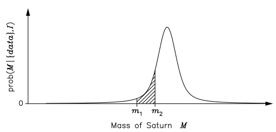
Although the frequency definition appears to be more objective, its range of validity is also far more limited. For example, Laplace used (his) probability theory to estimate the mass of Saturn, given orbital data that were available to him from various astronomical observatories. In essence, he computed the posterior pdf for the mass M , given the data and all the relevant background information I (such as a knowledge of the laws of classical mechanics): prob(M|{data},I); this is shown schematically in the figure [Fig. 1.2].

To Laplace, the (shaded) area under the posterior pdf curve between \( m_1 \) and \( m_2 \) was a measure of how much he believed that the mass of Saturn lay in the range \( m_1 \le M \le m_2 \). As such, the position of the maximum of the posterior pdf represents a best estimate of the mass; its width, or spread, about this optimal value gives an indication of the uncertainty in the estimate. Laplace stated that: ‘ . . . it is a bet of 11,000 to 1 that the error of this result is not 1/100th of its value.’ He would have won the bet, as another 150 years’ accumulation of data has changed the estimate by only 0.63%!
According to the frequency definition, however, we are not permitted to use probability theory to tackle this problem. This is because the mass of Saturn is a constant and not a random variable; therefore, it has no frequency distribution and so probability theory cannot be used.If the pdf [of Fig. 1.2] had to be interpreted in terms of the frequency definition, we would have to imagine a large ensemble of universes in which everything remains constant apart from the mass of Saturn.
As this scenario appears quite far-fetched, we might be inclined to think of [Fig. 1.2] in terms of the distribution of the measurements of the mass in many repetitions of the experiment. Although we are at liberty to think about a problem in any way that facilitates its solution, or our understanding of it, having to seek a frequency interpretation for every data analysis problem seems rather perverse. For example, what do we mean by the ‘measurement of the mass’ when the data consist of orbital periods? Besides, why should we have to think about many repetitions of an experiment that never happened? What we really want to do is to make the best inference of the mass given the (few) data that we actually have; this is precisely the Bayes and Laplace view of probability.
Faced with the realization that the frequency definition of probability theory did not permit most real-life scientific problems to be addressed, a new subject was invented — statistics! To estimate the mass of Saturn, for example, one has to relate the mass to the data through some function called the statistic; since the data are subject to ‘random’ noise, the statistic becomes the random variable to which the rules of probability the- ory can be applied. But now the question arises: How should we choose the statistic? The frequentist approach does not yield a natural way of doing this and has, therefore, led to the development of several alternative schools of orthodox or conventional statis- tics. The masters, such as Fisher, Neyman and Pearson, provided a variety of different principles, which has merely resulted in a plethora of tests and procedures without any clear underlying rationale. This lack of unifying principles is, perhaps, at the heart of the shortcomings of the cook-book approach to statistics that students are often taught even today.
Assess hypotheses by calculating their probabilities \( p(H_i | \ldots) \) conditional on known and/or presumed information using the rules of probability theory.
Probability Theory Axioms:
Bayes' theorem follows directly from the product rule $$ $$ p(A|B,I) = \frac{p(B|A,I) p(A|I)}{p(B|I)}. $$ $$ The importance of this property to data analysis becomes apparent if we replace \( A \) and \( B \) by hypothesis(\( H \)) and data(\( D \)): $$ \begin{align} p(H|D,I) &= \frac{p(D|H,I) p(H|I)}{p(D|I)}. \label{eq:bayes} \end{align} $$ The power of Bayes’ theorem lies in the fact that it relates the quantity of interest, the probability that the hypothesis is true given the data, to the term we have a better chance of being able to assign, the probability that we would have observed the measured data if the hypothesis was true.
The various terms in Bayes’ theorem have formal names.
In the continuum limit of propositions we must understand \( p(\ldots) \) as a pdf (probability density function).
Marginalization is a very powerful device in data analysis because it enables us to deal with nuisance parameters; that is, quantities which necessarily enter the analysis but are of no intrinsic interest. The unwanted background signal present in many experimental measurements are examples of nuisance parameters.
Inductive inference with parametric models is a very important tool in the natural sciences.
A sensible way of formulating this problem is to consider a large number of hypotheses about the range in which the bias-weighting of the coin might lie. If we denote the bias-weighting by \( H \), then \( H = 0 \) and \( H = 1 \) can represent a coin which produces a tail or a head on every flip, respectively. There is a continuum of possibilities for the value of H between these limits, with \( H = 0.5 \) indicating a fair coin. Our state of knowledge about the fairness, or the degree of unfairness, of the coin is then completely summarized by specifying how much we believe these various propositions to be true.
Let us perform a computer simulation of a coin-tossing experiment. This provides the data that we will be analysing.
import numpy as np
import matplotlib.pyplot as plt
np.random.seed(999)         # for reproducibility
a=0.6                       # biased coin
flips=np.random.rand(2**12) # simulates 4096 coin flips
heads=flips<a               # boolean array, heads[i]=True if flip i is heads
In the light of this data, our inference about the fairness of this coin is summarized by the conditional pdf: \( p(H|D,I) \). This is, of course, shorthand for the limiting case of a continuum of propositions for the value of \( H \); that is to say, the probability that \( H \) lies in an infinitesimally narrow range is given by \( p(H|D,I) dH \).
To estimate this posterior pdf, we need to use Bayes’ theorem \eqref{eq:bayes}. We will ignore the denominator \( p(D|I) \) as it does not involve bias-weighting explicitly, and it will therefore not affect the shape of the desired pdf. At the end we can evaluate the missing constant subsequently from the normalization condition $$ \begin{equation} \int_0^1 p(H|D,I) dH = 1. \label{eq:coin_posterior_norm} \end{equation} $$
The prior pdf, \( p(H|I) \), represents what we know about the coin given only the information \( I \) that we are dealing with a ‘strange coin’. We could keep a very open mind about the nature of the coin; a simple probability assignment which reflects this is a uniform, or flat, prior $$ \begin{equation} p(H|I) = \left\{ \begin{array}{ll} 1 & 0 \le H \le 1, \\ 0 & \mathrm{otherwise}. \end{array} \right. \label{eq:coin_prior_uniform} \end{equation} $$ We will get back later to the choice of prior and its effect on the analysis.
This prior state of knowledge, or ignorance, is modified by the data through the likelihood function \( p(D|H,I) \). It is a measure of the chance that we would have obtained the data that we actually observed, if the value of the bias-weighting was given (as known). If, in the conditioning information \( I \), we assume that the flips of the coin were independent events, so that the outcome of one did not influence that of another, then the probability of obtaining the data `R heads in N tosses' is given by the binomial distribution (we leave a formal definition of this to a statistics textbook) $$ \begin{equation} p(D|H,I) \propto H^R (1-H)^{N-R}. \label{_auto1} \end{equation} $$ It seems reasonable because \( H \) is the chance of obtaining a head on any flip, and there were \( R \) of them, and \( 1-H \) is the corresponding probability for a tail, of which there were \( N-R \). We note that this binomial distribution also contains a normalization factor, but we will ignore it since it does not depend explicitly on \( H \), the quantity of interest. It will be absorbed by the normalization condition \eqref{eq:coin_posterior_norm}.
We perform the setup of this Bayesian framework on the computer.
def prior(H):
    p=np.zeros_like(H)
    p[(0<=x)&(x<=1)]=1      # allowed range: 0<=H<=1
    return p                # uniform prior
def likelihood(H,data):
    N = len(data)
    no_of_heads = sum(data)
    no_of_tails = N - no_of_heads
    return H**no_of_heads * (1-H)**no_of_tails
def posterior(H,data):
    p=prior(H)*likelihood(H,data)
    norm=np.trapz(p,H)
    return p/norm
The next step is to confront this setup with the simulated data. To get a feel for the result, it is instructive to see how the posterior pdf evolves as we obtain more and more data pertaining to the coin. The results of such an analyses is shown in Fig. 1.
x=np.linspace(0,1,100)
fig, axs = plt.subplots(nrows=4,ncols=3,sharex=True,sharey='row')
axs_vec=np.reshape(axs,-1)
axs_vec[0].plot(x,prior(x))
for ndouble in range(11):
    ax=axs_vec[1+ndouble]
    ax.plot(x,posterior(x,heads[:2**ndouble]))
    ax.text(0.1, 0.8, '$N={0}$'.format(2**ndouble), transform=ax.transAxes)
for row in range(4): axs[row,0].set_ylabel('$p(H|D_\mathrm{obs},I)$')
for col in range(3): axs[-1,col].set_xlabel('$H$')
Figure 1: The evolution of the posterior pdf for the bias-weighting of a coin, as the number of data available increases. The figure on the top left-hand corner of each panel shows the number of data included in the analysis.
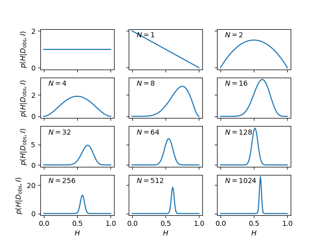
The panel in the top left-hand corner shows the posterior pdf for \( H \) given no data, i.e., it is the same as the prior pdf of Eq. \eqref{eq:coin_prior_uniform}. It indicates that we have no more reason to believe that the coin is fair than we have to think that it is double-headed, double-tailed, or of any other intermediate bias-weighting.
The first flip is obviously tails. At this point we have no evidence that the coin has a side with heads, as indicated by the pdf going to zero as \( H \to 1 \). The second flip is obviously heads and we have now excluded both extreme options \( H=0 \) (double-tailed) and \( H=1 \) (double-headed). We can note that the posterior at this point has the simple form \( p(H|D,I) = H(1-H) \) for \( 0 \le H \le 1 \).
The remainder of Fig. 1 shows how the posterior pdf evolves as the number of data analysed becomes larger and larger. We see that the position of the maximum moves around, but that the amount by which it does so decreases with the increasing number of observations. The width of the posterior pdf also becomes narrower with more data, indicating that we are becoming increasingly confident in our estimate of the bias-weighting. For the coin in this example, the best estimate of \( H \) eventually converges to 0.6, which, of course, was the value chosen to simulate the flips.
We will now consider the very important task of model parameter estimation using statistical inference. (CF 1: maybe stress that model parameters are not random variables, and the meaning of parameter estimation is therefore very different between frequentist and bayesian approaches.)
Throughout this section we will consider a specific example that involves a model with a single parameter: "Measured flux from a star".
Imagine that we point our telescope to the sky, and observe the light coming from a single star. For the time being, we'll assume that the star's true flux is constant with time, i.e. that is it has a fixed value \( F_\mathrm{true} \) (we'll also ignore effects like sky noise and other sources of systematic error). We'll assume that we perform a series of \( N \) measurements with our telescope, where the ith measurement reports the observed photon flux \( F_i \) and error \( e_i \) [2]. The question is, given this set of measurements \( D = \{F_i, e_i\} \), what is our best estimate of the true flux \( F_\mathrm{true} \)?
2: We'll make the reasonable assumption that errors are Gaussian. In a Frequentist perspective, \( e_i \) is the standard deviation of the results of a single measurement event in the limit of repetitions of that event. In the Bayesian perspective, \( e_i \) is the standard deviation of the (Gaussian) probability distribution describing our knowledge of that particular measurement given its observed value.
Because the measurements are number counts, a Poisson distribution is a good approximation to the measurement process:
np.random.seed(1)      # for repeatability
F_true = 1000          # true flux, say number of photons measured in 1 second
N = 50                 # number of measurements
F = stats.poisson(F_true).rvs(N)
                       # N measurements of the flux
e = np.sqrt(F)         # errors on Poisson counts estimated via square root
Now let's make a simple visualization of the "observed" data, see Fig. 2.
fig, ax = plt.subplots()
ax.errorbar(F, np.arange(N), xerr=e, fmt='ok', ecolor='gray', alpha=0.5)
ax.vlines([F_true], 0, N, linewidth=5, alpha=0.2)
ax.set_xlabel("Flux");ax.set_ylabel("measurement number");
Figure 2: Single photon counts (flux measurements).
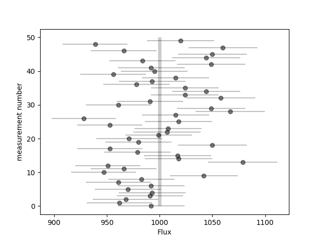
These measurements each have a different error \( e_i \) which is estimated from Poisson statistics using the standard square-root rule. In this toy example we already know the true flux \( F_\mathrm{true} \), but the question is this: given our measurements and errors, what is our best estimate of the true flux?
Let's take a look at the frequentist and Bayesian approaches to solving this.
We construct the likelihood function by computing the product of the probabilities for each data point $$ \begin{equation} \mathcal{L}(D | F_\mathrm{true}, I) = \prod_{i=1}^N p(D_i | F_\mathrm{true}, I), \label{_auto3} \end{equation} $$ here \( D = \{D_i\} \) represents the entire set of measurements. Because the value of the likelihood can become very small, it is often more convenient to instead compute the log-likelihood. Combining the previous two equations and computing the log, we have $$ \begin{equation} \log\mathcal{L} = -\frac{1}{2} \sum_{i=1}^N \left[ \log(2\pi e_i^2) + \frac{(F_i-F_\mathrm{true})^2}{e_i^2} \right]. \label{_auto4} \end{equation} $$
What we'd like to do is determine \( F_\mathrm{true} \) such that the likelihood is maximized. For this simple problem, the maximization can be computed analytically (i.e. by setting \( d\log\mathcal{L}/d F_\mathrm{true} = 0 \)). This results in the following observed estimate of \( F_\mathrm{true} \) $$ \begin{equation} F_\mathrm{est} = \sum_{i=1}^N w_i F_i; \quad w_i = 1/e_i^2. \label{_auto5} \end{equation} $$ Notice that in the special case of all errors \( e_i \) being equal, this reduces to $$ \begin{equation} F_\mathrm{est} = \frac{1}{N} \sum_{i=1} F_i. \label{_auto6} \end{equation} $$ That is, in agreement with intuition, \( F_\mathrm{est} \) is simply the mean of the observed data when errors are equal.
We can go further and ask what the error of our estimate is. In the frequentist approach, this can be accomplished by fitting a Gaussian approximation to the likelihood curve at maximum; in this simple case this can also be solved analytically (the sum of Gaussians is also a Gaussian). It can be shown that the standard deviation of this Gaussian approximation is $$ \begin{equation} \sigma_\mathrm{est} = \sum_{i=1}^N w_i. \label{_auto7} \end{equation} $$ These results are fairly simple calculations; let's evaluate them for our toy dataset:
w=1./e**2
print("""
F_true = {0}
F_est = {1:.0f} +/- {2:.0f} (based on {3} measurements) """\
          .format(F_true, (w * F).sum() / w.sum(), w.sum() ** -0.5, N))
F_true = 1000
F_est = 998 +/- 4 (based on 50 measurements)
We find that for 50 measurements of the flux, our estimate has an error of about 0.4% and is consistent with the input value.
To compute this result, Bayesians next apply Bayes' Theorem \eqref{eq:bayes}. If we set the prior \( p(F_\mathrm{true}|I) \propto 1 \) (a flat prior), we find \( p(F_\mathrm{true}|D,I) \propto p(D | F_\mathrm{true},I) \equiv \mathcal{L}(D | F_\mathrm{true},I) \) and the Bayesian probability is maximized at precisely the same value as the frequentist result! So despite the philosophical differences, we see that (for this simple problem at least) the Bayesian and frequentist point estimates are equivalent.
def log_prior(alpha):
    return 0 # flat prior

def log_likelihood(alpha, F, e):
    return -0.5 * np.sum(np.log(2 * np.pi * e ** 2) \
                             + (F - alpha[0]) ** 2 / e ** 2)

def log_posterior(alpha, F, e):
    return log_prior(alpha) + log_likelihood(alpha, F, e)
Now we set up the problem, including generating some random starting guesses for the multiple chains of points.
ndim = 1      # number of parameters in the model
nwalkers = 50 # number of MCMC walkers
nburn = 1000  # "burn-in" period to let chains stabilize
nsteps = 2000 # number of MCMC steps to take
# we'll start at random locations between 0 and 2000
starting_guesses = 2000 * np.random.rand(nwalkers, ndim)
sampler = emcee.EnsembleSampler(nwalkers, ndim, log_posterior, args=[F,e])
sampler.run_mcmc(starting_guesses, nsteps)
# Shape of sampler.chain  = (nwalkers, nsteps, ndim)
# Flatten the sampler chain and discard burn-in points:
samples = sampler.chain[:, nburn:, :].reshape((-1, ndim))
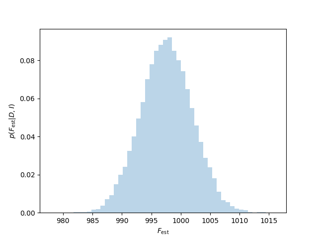
If this all worked correctly, the array sample should contain a series of 50,000 points drawn from the posterior. Let's plot them and check. See results in Fig. 3.
fig, ax = plt.subplots()
ax.hist(samples, bins=50, histtype="stepfilled", alpha=0.3, normed=True)
ax.set_xlabel(r'$F_\mathrm{est}$')
ax.set_ylabel(r'$p(F_\mathrm{est}|D,I)$')
Figure 3: Bayesian posterior pdf (represented by a histogram of MCMC samples) from flux measurements.
There are a few different options for this. The choice of the most appropriate one depends mainly on the shape of the posterior distribution:
Symmetric posterior pdfs: Since the probability (density) associated with any particular value of the parameter is a measure of how much we believe that it lies in the neighbourhood of that point, our best estimate is given by the maximum of the posterior pdf. If we denote the quantity of interest by \( X \), with a posterior pdf \( P =p(X|D,I) \), then the best estimate of its value \( X_0 \) is given by the condition \( dP/dX|_{X=X_0}=0 \). Strictly speaking, we should also check the sign of the second derivative to ensure that \( X_0 \) represents a maximum.
To obtain a measure of the reliability of this best estimate, we need to look at the width or spread of the posterior pdf about \( X_0 \). When considering the behaviour of any function in the neighbourhood of a particular point, it is often helpful to carry out a Taylor series expansion; this is simply a standard tool for (locally) approximating a complicated function by a low-order polynomial. The linear term is zero at the maximum and the quadratic term is often the dominating one determining the width of the posterior pdf. Ignoring all the higher-order terms we arrive at the Gaussian approximation $$ \begin{equation} p(X|D,I) \approx \frac{1}{\sigma\sqrt{2\pi}} \exp \left[ -\frac{(x-\mu)^2}{2\sigma^2} \right], \label{_auto8} \end{equation} $$ where the mean \( \mu = X_0 \) and the variance \( \sigma = \left( - \left. \frac{d^2L}{dX^2} \right|_{X_0} \right)^{-1/2} \), where \( L \) is the logarithm of the posterior \( P \). Our inference about the quantity of interest is conveyed very concisely, therefore, by the statement \( X = X_0 \pm \sigma \), and $$ $$ p(X_0-\sigma < X < X_0+\sigma | D,I) = \int_{X_0-\sigma}^{X_0+\sigma} p(X|D,I) dX \approx 0.67. $$ $$
Asymmetric posterior pdfs: While the maximum of the posterior (\( X_0 \)) can still be regarded as giving the best estimate, the true value is now more likely to be on one side of this rather than the other. Alternatively one can compute the mean value, \( \langle X \rangle = \int X p(X|D,I) dX \), although this tends to overemphasise very long tails. The best option is probably a compromise that can be employed when having access to a large sample from the posterior (as provided by an MCMC), namely to give the median of this ensamble.
Furthermore, the concept of an error-bar does not seem appropriate in this case, as it implicitly entails the idea of symmetry. A good way of expressing the reliability with which a parameter can be inferred, for an asymmetric posterior pdf, is rather through a confidence interval. Since the area under the posterior pdf between \( X_1 \) and \( X_2 \) is proportional to how much we believe that \( X \) lies in that range, the shortest interval that encloses 67% of the area represents a sensible measure of the uncertainty of the estimate. Obviously we can choose to provide some other degree-of-belief that we think is relevant for the case at hand. Assuming that the posterior pdf has been normalized, to have unit area, we need to find \( X_1 \) and \( X_2 \) such that: $$ $$ p(X_1 < X < X_2 | D,I) = \int_{X_1}^{X_2} p(X|D,I) dX \approx 0.67, $$ $$ where the difference \( X_2 - X_1 \) is as small as possible. The region \( X_1 < X < X_2 \) is then called the shortest 67% confidence interval.
Multimodal posterior pdfs: We can sometimes obtain posteriors which are multimodal; i.e. contains several disconnected regions with large probabilities. There is no difficulty when one of the maxima is very much larger than the others: we can simply ignore the subsidiary solutions, to a good approximation, and concentrate on the global maximum. The problem arises when there are several maxima of comparable magnitude. What do we now mean by a best estimate, and how should we quantify its reliability? The idea of a best estimate and an error-bar, or even a confidence interval, is merely an attempt to summarize the posterior with just two or three numbers; sometimes this just can’t be done, and so these concepts are not valid. For the bimodal case we might be able to characterize the posterior in terms of a few numbers: two best estimates and their associated error-bars, or disjoint confidence intervals. For a general multimodal pdf, the most honest thing we can do is just display the posterior itself.
sampper=np.percentile(samples, [2.5, 16.5, 50, 83.5, 97.5],axis=0).flatten()
print("""
F_true = {0}
Based on {1} measurements the posterior point estimates are:
...F_est = {2:.0f} +/- {3:.0f}
or using credible intervals:
...F_est = {4:.0f}          (posterior median)
...F_est in [{5:.0f}, {6:.0f}] (67% credible interval)
...F_est in [{7:.0f}, {8:.0f}] (95% credible interval) """\
          .format(F_true, N, np.mean(samples), np.std(samples), \
                      sampper[2], sampper[1], sampper[3], sampper[0], sampper[4]))
F_true = 1000
Based on 50 measurements the posterior point estimates are:
...F_est = 998 +/- 4
or using credible intervals:
...F_est = 998 (posterior median)
...F_est in [993, 1002] (67% credible interval)
...F_est in [989, 1006] (95% credible interval)
In this particular example, the posterior pdf is actually a Gaussian (since it is constructed as a product of Gaussians), and the mean and variance from the quadratic approximation will agree exactly with the frequentist approach.
From this final result you might come away with the impression that the Bayesian method is unnecessarily complicated, and in this case it certainly is. Using an MCMC sampler to characterize a one-dimensional normal distribution is a bit like using the Death Star to destroy a beach ball, but we did this here because it demonstrates an approach that can scale to complicated posteriors in many, many dimensions, and can provide nice results in more complicated situations where an analytic likelihood approach is not possible.
Furthermore, as data and models grow in complexity, the two approaches can diverge greatly.