.ipynb .pdf

Contents

7. Resampling Techniques, Bootstrap and Blocking

7.1. Why resampling methods ?

Statistical analysis.

* Our simulations can be treated as *computer experiments*. This is particularly the case for Monte Carlo methods

* The results can be analysed with the same statistical tools as we would use analysing experimental data.

* As in all experiments, we are looking for expectation values and an estimate of how accurate they are, i.e., possible sources for errors.

7.2. Statistical analysis

* As in other experiments, many numerical  experiments have two classes of errors:

  * Statistical errors

  * Systematical errors


* Statistical errors can be estimated using standard tools from statistics

* Systematical errors are method specific and must be treated differently from case to case.

7.3. Statistics, wrapping up from last week

Let us analyze the problem by splitting up the correlation term into partial sums of the form:

$$f_d=\frac{1}{n-d}\sum _{k=1}^{n-d}(x_k-{\overline{x}}_n)(x_{k+d}-{\overline{x}}_n)$$

The correlation term of the error can now be rewritten in terms of $f_d$

$$\frac{2}{n}\sum _{k<l}(x_k-{\overline{x}}_n)(x_l-{\overline{x}}_n)=2\sum _{d=1}^{n-1}{f}_d$$

The value of $f_d$ reflects the correlation between measurements separated by the distance $d$ in the sample samples. Notice that for $d=0$, $f$ is just the sample variance, $\mathrm{var}(x)$. If we divide $f_d$ by $\mathrm{var}(x)$, we arrive at the so called autocorrelation function

$${\kappa }_d=\frac{f_d}{\mathrm{var}(x)}$$

which gives us a useful measure of pairwise correlations starting always at $1$ for $d=0$.

7.4. Statistics, final expression

The sample error can now be written in terms of the autocorrelation function:

$$\begin{array}{}& {\mathrm{err}}_X^2=\frac{1}{n}\mathrm{var}(x)+\frac{2}{n}\cdot \mathrm{var}(x)\sum _{d=1}^{n-1}\frac{f_d}{\mathrm{var}(x)}\end{array}$$

$$\begin{array}{}& =(1+2\sum _{d=1}^{n-1}{\kappa }_d)\frac{1}{n}\mathrm{var}(x)\end{array}$$

$$\begin{array}{}\text{(1)}& =\frac{\tau }{n}\cdot \mathrm{var}(x)\end{array}$$

and we see that ${\mathrm{err}}_X$ can be expressed in terms the uncorrelated sample variance times a correction factor $\tau$ which accounts for the correlation between measurements. We call this correction factor the autocorrelation time:

$$\begin{array}{}\text{(2)}& \tau =1+2\sum _{d=1}^{n-1}{\kappa }_d\end{array}$$

7.5. Statistics, effective number of correlations

For a correlation free experiment, $\tau$ equals 1.

We can interpret a sequential correlation as an effective reduction of the number of measurements by a factor $\tau$. The effective number of measurements becomes:

$$n_{\mathrm{eff}}=\frac{n}{\tau }$$

To neglect the autocorrelation time $\tau$ will always cause our simple uncorrelated estimate of ${\mathrm{err}}_X^2\approx \mathrm{var}(x)/n$ to be less than the true sample error. The estimate of the error will be too good. On the other hand, the calculation of the full autocorrelation time poses an efficiency problem if the set of measurements is very large.

7.6. Can we understand this? Time Auto-correlation Function

The so-called time-displacement autocorrelation $\varphi (t)$ for a quantity $\mathbf{M}$ is given by

$$\varphi (t)=\int d{t}^{\prime }[\mathbf{M}(t^{\prime })-⟨\mathbf{M}⟩][\mathbf{M}(t^{\prime }+t)-⟨\mathbf{M}⟩],$$

which can be rewritten as

$$\varphi (t)=\int d{t}^{\prime }[\mathbf{M}(t^{\prime })\mathbf{M}(t^{\prime }+t)-⟨\mathbf{M}{⟩}^2],$$

where $⟨\mathbf{M}⟩$ is the average value and $\mathbf{M}(t)$ its instantaneous value. We can discretize this function as follows, where we used our set of computed values $\mathbf{M}(t)$ for a set of discretized times (our Monte Carlo cycles corresponding to moving all electrons?)

$$\begin{array}{}\text{(3)}& \varphi (t)=\frac{1}{t_{\max }-t}\sum _{t^{\prime }=0}^{t_{\max }-t}\mathbf{M}(t^{\prime })\mathbf{M}(t^{\prime }+t)-\frac{1}{t_{\max }-t}\sum _{t^{\prime }=0}^{t_{\max }-t}\mathbf{M}(t^{\prime })\times \frac{1}{t_{\max }-t}\sum _{t^{\prime }=0}^{t_{\max }-t}\mathbf{M}(t^{\prime }+t).\end{array}$$

7.7. Time Auto-correlation Function

One should be careful with times close to $t_{\max }$, the upper limit of the sums becomes small and we end up integrating over a rather small time interval. This means that the statistical error in $\varphi (t)$ due to the random nature of the fluctuations in $\mathbf{M}(t)$ can become large.

One should therefore choose $t\ll t_{\max }$.

Note that the variable $\mathbf{M}$ can be any expectation values of interest.

The time-correlation function gives a measure of the correlation between the various values of the variable at a time $t^{\prime }$ and a time $t^{\prime }+t$. If we multiply the values of $\mathbf{M}$ at these two different times, we will get a positive contribution if they are fluctuating in the same direction, or a negative value if they fluctuate in the opposite direction. If we then integrate over time, or use the discretized version of, the time correlation function $\varphi (t)$ should take a non-zero value if the fluctuations are correlated, else it should gradually go to zero. For times a long way apart the different values of $\mathbf{M}$ are most likely uncorrelated and $\varphi (t)$ should be zero.

7.8. Time Auto-correlation Function

We can derive the correlation time by observing that our Metropolis algorithm is based on a random walk in the space of all possible spin configurations. Our probability distribution function $\hat{\mathbf{w}}(t)$ after a given number of time steps $t$ could be written as

$$\hat{\mathbf{w}}(t)={\hat{\mathbf{W}}}^{\mathbf{t}}\hat{\mathbf{w}}(0),$$

with $\hat{\mathbf{w}}(0)$ the distribution at $t=0$ and $\hat{\mathbf{W}}$ representing the transition probability matrix. We can always expand $\hat{\mathbf{w}}(0)$ in terms of the right eigenvectors of $\hat{\mathbf{v}}$ of $\hat{\mathbf{W}}$ as

$$\hat{\mathbf{w}}(0)=\sum _i{\alpha }_i{\hat{\mathbf{v}}}_i,$$

resulting in

$$\hat{\mathbf{w}}(t)={\hat{\mathbf{W}}}^t\hat{\mathbf{w}}(0)={\hat{\mathbf{W}}}^t\sum _i{\alpha }_i{\hat{\mathbf{v}}}_i=\sum _i{\lambda }_i^t{\alpha }_i{\hat{\mathbf{v}}}_i,$$

with ${\lambda }_i$ the $i^{\mathrm{th}}$ eigenvalue corresponding to
the eigenvector ${\hat{\mathbf{v}}}_i$.

7.9. Time Auto-correlation Function

If we assume that ${\lambda }_0$ is the largest eigenvector we see that in the limit $t\to \mathrm{\infty }$, $\hat{\mathbf{w}}(t)$ becomes proportional to the corresponding eigenvector ${\hat{\mathbf{v}}}_0$. This is our steady state or final distribution.

We can relate this property to an observable like the mean energy. With the probabilty $\hat{\mathbf{w}}(t)$ (which in our case is the squared trial wave function) we can write the expectation values as

$$⟨\mathbf{M}(t)⟩=\sum _{\mu }\hat{\mathbf{w}}(t{)}_{\mu }{\mathbf{M}}_{\mu },$$

or as the scalar of a vector product

$$⟨\mathbf{M}(t)⟩=\hat{\mathbf{w}}(t)\mathbf{m},$$

with $\mathbf{m}$ being the vector whose elements are the values of ${\mathbf{M}}_{\mu }$ in its various microstates $\mu$.

7.10. Time Auto-correlation Function

We rewrite this relation as

$$⟨\mathbf{M}(t)⟩=\hat{\mathbf{w}}(t)\mathbf{m}=\sum _i{\lambda }_i^t{\alpha }_i{\hat{\mathbf{v}}}_i{\mathbf{m}}_i.$$

If we define $m_i={\hat{\mathbf{v}}}_i{\mathbf{m}}_i$ as the expectation value of $\mathbf{M}$ in the $i^{\mathrm{th}}$ eigenstate we can rewrite the last equation as

$$⟨\mathbf{M}(t)⟩=\sum _i{\lambda }_i^t{\alpha }_i{m}_i.$$

Since we have that in the limit $t\to \mathrm{\infty }$ the mean value is dominated by the the largest eigenvalue ${\lambda }_0$, we can rewrite the last equation as

$$⟨\mathbf{M}(t)⟩=⟨\mathbf{M}(\mathrm{\infty })⟩+\sum _{i\ne 0}{\lambda }_i^t{\alpha }_i{m}_i.$$

We define the quantity

$${\tau }_i=-\frac{1}{log{\lambda }_i},$$

and rewrite the last expectation value as

$$\begin{array}{}\text{(4)}& ⟨\mathbf{M}(t)⟩=⟨\mathbf{M}(\mathrm{\infty })⟩+\sum _{i\ne 0}{\alpha }_i{m}_i{e}^{-t/{\tau }_i}.\end{array}$$

7.11. Time Auto-correlation Function

The quantities ${\tau }_i$ are the correlation times for the system. They control also the auto-correlation function discussed above. The longest correlation time is obviously given by the second largest eigenvalue ${\tau }_1$, which normally defines the correlation time discussed above. For large times, this is the only correlation time that survives. If higher eigenvalues of the transition matrix are well separated from ${\lambda }_1$ and we simulate long enough, ${\tau }_1$ may well define the correlation time. In other cases we may not be able to extract a reliable result for ${\tau }_1$. Coming back to the time correlation function $\varphi (t)$ we can present a more general definition in terms of the mean magnetizations $⟨\mathbf{M}(t)⟩$. Recalling that the mean value is equal to $⟨\mathbf{M}(\mathrm{\infty })⟩$ we arrive at the expectation values

$$\varphi (t)=⟨\mathbf{M}(0)-\mathbf{M}(\mathrm{\infty })⟩⟨\mathbf{M}(t)-\mathbf{M}(\mathrm{\infty })⟩,$$

resulting in

$$\varphi (t)=\sum _{i,j\ne 0}{m}_i{\alpha }_i{m}_j{\alpha }_j{e}^{-t/{\tau }_i},$$

which is appropriate for all times.

7.12. Correlation Time

If the correlation function decays exponentially

$$\varphi (t)\sim \exp (-t/\tau )$$

then the exponential correlation time can be computed as the average

$${\tau }_{\exp }=-⟨\frac{t}{log|\frac{\varphi (t)}{\varphi (0)}|}⟩.$$

If the decay is exponential, then

$${\int }_0^{\mathrm{\infty }}dt\varphi (t)={\int }_0^{\mathrm{\infty }}dt\varphi (0)\exp (-t/\tau )=\tau \varphi (0),$$

which suggests another measure of correlation

$${\tau }_{\mathrm{int}}=\sum _k\frac{\varphi (k)}{\varphi (0)},$$

called the integrated correlation time.

7.13. Resampling methods: Jackknife and Bootstrap

Two famous resampling methods are the independent bootstrap and the jackknife.

The jackknife is a special case of the independent bootstrap. Still, the jackknife was made popular prior to the independent bootstrap. And as the popularity of the independent bootstrap soared, new variants, such as the dependent bootstrap.

The Jackknife and independent bootstrap work for independent, identically distributed random variables. If these conditions are not satisfied, the methods will fail. Yet, it should be said that if the data are independent, identically distributed, and we only want to estimate the variance of $\bar{X}$ (which often is the case), then there is no need for bootstrapping.

7.14. Resampling methods: Jackknife

The Jackknife works by making many replicas of the estimator $\hat{\theta }$. The jackknife is a resampling method, we explained that this happens by scrambling the data in some way. When using the jackknife, this is done by systematically leaving out one observation from the vector of observed values $\hat{x}=(x_1,x_2,\cdots ,X_n)$. Let ${\hat{x}}_i$ denote the vector

$${\hat{x}}_i=(x_1,x_2,\cdots ,x_{i-1},x_{i+1},\cdots ,x_n),$$

which equals the vector $\hat{x}$ with the exception that observation number $i$ is left out. Using this notation, define ${\hat{\theta }}_i$ to be the estimator $\hat{\theta }$ computed using ${\overrightarrow{X}}_i$.

7.15. Resampling methods: Jackknife estimator

To get an estimate for the bias and standard error of $\hat{\theta }$, use the following estimators for each component of $\hat{\theta }$

$$\widehat{\mathrm{Bias}}(\hat{\theta },\theta )=(n-1)(-\hat{\theta }+\frac{1}{n}\sum _{i=1}^n{\hat{\theta }}_i)\text{and}{\hat{\sigma }}_{\hat{\theta }}^2=\frac{n-1}{n}\sum _{i=1}^n({\hat{\theta }}_i-\frac{1}{n}\sum _{j=1}^n{\hat{\theta }}_j{)}^2.$$

7.16. Jackknife code example

from numpy import *
from numpy.random import randint, randn
from time import time

def jackknife(data, stat):
    n = len(data);t = zeros(n); inds = arange(n); t0 = time()
    ## 'jackknifing' by leaving out an observation for each i                                                                                                                      
    for i in range(n):
        t[i] = stat(delete(data,i) )

    # analysis                                                                                                                                                                     
    print("Runtime: %g sec" % (time()-t0)); print("Jackknife Statistics :")
    print("original           bias      std. error")
    print("%8g %14g %15g" % (stat(data),(n-1)*mean(t)/n, (n*var(t))**.5))

    return t


# Returns mean of data samples                                                                                                                                                     
def stat(data):
    return mean(data)


mu, sigma = 100, 15
datapoints = 10000
x = mu + sigma*random.randn(datapoints)
# jackknife returns the data sample                                                                                                                                                
t = jackknife(x, stat)

Runtime: 0.0904138 sec
Jackknife Statistics :
original           bias      std. error
 99.9498        99.9399        0.151413

7.17. Resampling methods: Bootstrap

Bootstrapping is a nonparametric approach to statistical inference that substitutes computation for more traditional distributional assumptions and asymptotic results. Bootstrapping offers a number of advantages:

1. The bootstrap is quite general, although there are some cases in which it fails.

2. Because it does not require distributional assumptions (such as normally distributed errors), the bootstrap can provide more accurate inferences when the data are not well behaved or when the sample size is small.

3. It is possible to apply the bootstrap to statistics with sampling distributions that are difficult to derive, even asymptotically.

4. It is relatively simple to apply the bootstrap to complex data-collection plans (such as stratified and clustered samples).

7.18. Resampling methods: Bootstrap background

Since $\hat{\theta }=\hat{\theta }(\hat{X})$ is a function of random variables, $\hat{\theta }$ itself must be a random variable. Thus it has a pdf, call this function $p(\hat{t})$. The aim of the bootstrap is to estimate $p(\hat{t})$ by the relative frequency of $\hat{\theta }$. You can think of this as using a histogram in the place of $p(\hat{t})$. If the relative frequency closely resembles $p(\overrightarrow{t})$, then using numerics, it is straight forward to estimate all the interesting parameters of $p(\hat{t})$ using point estimators.

7.19. Resampling methods: More Bootstrap background

In the case that $\hat{\theta }$ has more than one component, and the components are independent, we use the same estimator on each component separately. If the probability density function of $X_i$, $p(x)$, had been known, then it would have been straight forward to do this by:

1. Drawing lots of numbers from $p(x)$, suppose we call one such set of numbers $(X_1^{\ast },X_2^{\ast },\cdots ,X_n^{\ast })$.

2. Then using these numbers, we could compute a replica of $\hat{\theta }$ called ${\hat{\theta }}^{\ast }$.

By repeated use of (1) and (2), many estimates of $\hat{\theta }$ could have been obtained. The idea is to use the relative frequency of ${\hat{\theta }}^{\ast }$ (think of a histogram) as an estimate of $p(\hat{t})$.

7.20. Resampling methods: Bootstrap approach

But unless there is enough information available about the process that generated $X_1,X_2,\cdots ,X_n$, $p(x)$ is in general unknown. Therefore, Efron in 1979 asked the question: What if we replace $p(x)$ by the relative frequency of the observation $X_i$; if we draw observations in accordance with the relative frequency of the observations, will we obtain the same result in some asymptotic sense? The answer is yes.

Instead of generating the histogram for the relative frequency of the observation $X_i$, just draw the values $(X_1^{\ast },X_2^{\ast },\cdots ,X_n^{\ast })$ with replacement from the vector $\hat{X}$.

7.21. Resampling methods: Bootstrap steps

The independent bootstrap works like this:

1. Draw with replacement $n$ numbers for the observed variables $\hat{x}=(x_1,x_2,\cdots ,x_n)$.

2. Define a vector ${\hat{x}}^{\ast }$ containing the values which were drawn from $\hat{x}$.

3. Using the vector ${\hat{x}}^{\ast }$ compute ${\hat{\theta }}^{\ast }$ by evaluating $\hat{\theta }$ under the observations ${\hat{x}}^{\ast }$.

4. Repeat this process $k$ times.

When you are done, you can draw a histogram of the relative frequency of ${\hat{\theta }}^{\ast }$. This is your estimate of the probability distribution $p(t)$. Using this probability distribution you can estimate any statistics thereof. In principle you never draw the histogram of the relative frequency of ${\hat{\theta }}^{\ast }$. Instead you use the estimators corresponding to the statistic of interest. For example, if you are interested in estimating the variance of $\hat{\theta }$, apply the etsimator ${\hat{\sigma }}^2$ to the values ${\hat{\theta }}^{\ast }$.

7.22. Code example for the Bootstrap method

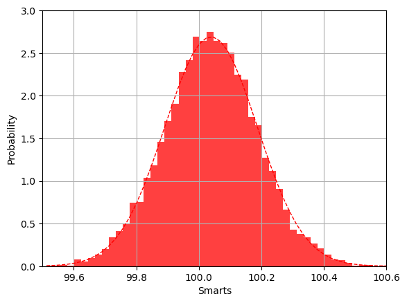
The following code starts with a Gaussian distribution with mean value $\mu =100$ and variance $\sigma =15$. We use this to generate the data used in the bootstrap analysis. The bootstrap analysis returns a data set after a given number of bootstrap operations (as many as we have data points). This data set consists of estimated mean values for each bootstrap operation. The histogram generated by the bootstrap method shows that the distribution for these mean values is also a Gaussian, centered around the mean value $\mu =100$ but with standard deviation $\sigma /\sqrt{n}$, where $n$ is the number of bootstrap samples (in this case the same as the number of original data points). The value of the standard deviation is what we expect from the central limit theorem.

%matplotlib inline


%matplotlib inline

from numpy import *
from numpy.random import randint, randn
from time import time
from scipy.stats import norm
import matplotlib.pyplot as plt

# Returns mean of bootstrap samples                                                                                                                                                
def stat(data):
    return mean(data)

# Bootstrap algorithm                                                                                                                                                              
def bootstrap(data, statistic, R):
    t = zeros(R); n = len(data); inds = arange(n); t0 = time()

    # non-parametric bootstrap                                                                                                                                                     
    for i in range(R):
        t[i] = statistic(data[randint(0,n,n)])

    # analysis                                                                                                                                                                     
    print("Runtime: %g sec" % (time()-t0)); print("Bootstrap Statistics :")
    print("original           bias      std. error")
    print("%8g %8g %14g %15g" % (statistic(data), std(data),\
                             mean(t), \
                             std(t)))
    return t


mu, sigma = 100, 15
datapoints = 10000
x = mu + sigma*random.randn(datapoints)
# bootstrap returns the data sample                                                                                                          t = bootstrap(x, stat, datapoints)
# the histogram of the bootstrapped  data  
t = bootstrap(x, stat, datapoints)
# the histogram of the bootstrapped  data                                            
n, binsboot, patches = plt.hist(t, bins=50, density='true',histtype='bar', color='red', alpha=0.75)

# add a 'best fit' line                                                                                                                                                          
y = norm.pdf( binsboot, mean(t), std(t))
lt = plt.plot(binsboot, y, 'r--', linewidth=1)
plt.xlabel('Smarts')
plt.ylabel('Probability')
plt.axis([99.5, 100.6, 0, 3.0])
plt.grid(True)

plt.show()

Runtime: 1.23216 sec
Bootstrap Statistics :
original           bias      std. error
 100.039  14.8853        100.039        0.148237

7.23. Resampling methods: Blocking

The blocking method was made popular by Flyvbjerg and Pedersen (1989) and has become one of the standard ways to estimate $V(\hat{\theta })$ for exactly one $\hat{\theta }$, namely $\hat{\theta }=\bar{X}$.

Assume $n=2^d$ for some integer $d>1$ and $X_1,X_2,\cdots ,X_n$ is a stationary time series to begin with. Moreover, assume that the time series is asymptotically uncorrelated. We switch to vector notation by arranging $X_1,X_2,\cdots ,X_n$ in an $n$-tuple. Define:

$$\begin{array}{r}\hat{X}=(X_1,X_2,\cdots ,X_n).\end{array}$$

The strength of the blocking method is when the number of observations, $n$ is large. For large $n$, the complexity of dependent bootstrapping scales poorly, but the blocking method does not, moreover, it becomes more accurate the larger $n$ is.

7.24. Blocking Transformations

We now define blocking transformations. The idea is to take the mean of subsequent pair of elements from $\overrightarrow{X}$ and form a new vector ${\overrightarrow{X}}_1$. Continuing in the same way by taking the mean of subsequent pairs of elements of ${\overrightarrow{X}}_1$ we obtain ${\overrightarrow{X}}_2$, and so on. Define ${\overrightarrow{X}}_i$ recursively by:

$$\begin{array}{}& ({\overrightarrow{X}}_0{)}_k\equiv (\overrightarrow{X}{)}_k\end{array}$$

$$\begin{array}{}\text{(5)}& ({\overrightarrow{X}}_{i+1}{)}_k\equiv \frac{1}{2}(({\overrightarrow{X}}_i{)}_{2k-1}+({\overrightarrow{X}}_i{)}_{2k})\text{for all}1\le i\le d-1\end{array}$$

The quantity ${\overrightarrow{X}}_k$ is subject to $k$ blocking transformations. We now have $d$ vectors ${\overrightarrow{X}}_0,{\overrightarrow{X}}_1,\cdots ,{\overrightarrow{X}}_{d-1}$ containing the subsequent averages of observations. It turns out that if the components of $\overrightarrow{X}$ is a stationary time series, then the components of ${\overrightarrow{X}}_i$ is a stationary time series for all $0\le i\le d-1$

We can then compute the autocovariance, the variance, sample mean, and number of observations for each $i$. Let ${\gamma }_i,{\sigma }_i^2,{\bar{X}}_i$ denote the autocovariance, variance and average of the elements of ${\overrightarrow{X}}_i$ and let $n_i$ be the number of elements of ${\overrightarrow{X}}_i$. It follows by induction that $n_i=n/2^i$.

7.25. Blocking Transformations

Using the definition of the blocking transformation and the distributive property of the covariance, it is clear that since $h=|i-j|$ we can define

$$\begin{array}{}& {\gamma }_{k+1}(h)=cov((X_{k+1}{)}_i,(X_{k+1}{)}_j)\end{array}$$

$$\begin{array}{}& =\frac{1}{4}cov((X_k{)}_{2i-1}+(X_k{)}_{2i},(X_k{)}_{2j-1}+(X_k{)}_{2j})\end{array}$$

$$\begin{array}{}\text{(6)}& =\frac{1}{2}{\gamma }_k(2h)+\frac{1}{2}{\gamma }_k(2h+1)\mathrm{h}=0\end{array}$$

$$\begin{array}{}\text{(7)}& =\frac{1}{4}{\gamma }_k(2h-1)+\frac{1}{2}{\gamma }_k(2h)+\frac{1}{4}{\gamma }_k(2h+1)\mathrm{else}\end{array}$$

The quantity $\hat{X}$ is asymptotic uncorrelated by assumption, ${\hat{X}}_k$ is also asymptotic uncorrelated. Let’s turn our attention to the variance of the sample mean $V(\bar{X})$.

7.26. Blocking Transformations, getting there

We have

$$\begin{array}{}\text{(8)}& V({\bar{X}}_k)=\frac{{\sigma }_k^2}{n_k}+\underset{\equiv e_k}{\underbrace{\frac{2}{n_k}\sum _{h=1}^{n_k-1}(1-\frac{h}{n_k}){\gamma }_k(h)}}=\frac{{\sigma }_k^2}{n_k}+e_k\text{if}{\gamma }_k(0)={\sigma }_k^2.\end{array}$$

The term $e_k$ is called the truncation error:

$$\begin{array}{}\text{(9)}& e_k=\frac{2}{n_k}\sum _{h=1}^{n_k-1}(1-\frac{h}{n_k}){\gamma }_k(h).\end{array}$$

We can show that $V({\bar{X}}_i)=V({\bar{X}}_j)$ for all $0\le i\le d-1$ and $0\le j\le d-1$.

7.27. Blocking Transformations, final expressions

We can then wrap up

$$\begin{array}{}& n_{j+1}{\bar{X}}_{j+1}=\sum _{i=1}^{n_{j+1}}({\hat{X}}_{j+1}{)}_i=\frac{1}{2}\sum _{i=1}^{n_j/2}({\hat{X}}_j{)}_{2i-1}+({\hat{X}}_j{)}_{2i}\end{array}$$

$$\begin{array}{}\text{(10)}& =\frac{1}{2}[({\hat{X}}_j{)}_1+({\hat{X}}_j{)}_2+\cdots +({\hat{X}}_j{)}_{n_j}]=\underset{=n_{j+1}}{\underbrace{\frac{n_j}{2}}}{\bar{X}}_j=n_{j+1}{\bar{X}}_j.\end{array}$$

By repeated use of this equation we get $V({\bar{X}}_i)=V({\bar{X}}_0)=V(\bar{X})$ for all $0\le i\le d-1$. This has the consequence that

$$\begin{array}{}\text{(11)}& V(\bar{X})=\frac{{\sigma }_k^2}{n_k}+e_k\text{for all}0\le k\le d-1.\end{array}$$

Flyvbjerg and Petersen demonstrated that the sequence $\{e_k{\}}_{k=0}^{d-1}$ is decreasing, and conjecture that the term $e_k$ can be made as small as we would like by making $k$ (and hence $d$) sufficiently large. The sequence is decreasing (Master of Science thesis by Marius Jonsson, UiO 2018). It means we can apply blocking transformations until $e_k$ is sufficiently small, and then estimate $V(\bar{X})$ by ${\hat{\sigma }}_k^2/n_k$.

For an elegant solution and proof of the blocking method, see the recent article of Marius Jonsson (former MSc student of the Computational Physics group).

previous

6. Gradient Methods

next

8. Optimization and Vectorization