Week 42 Constructing a Neural Network code with examples
Contents
Lecture October 13, 2025
Readings and videos
Material for the lab sessions on Tuesday and Wednesday
Lecture material: Writing a code which implements a feed-forward neural network
Mathematics of deep learning
Reminder on books with hands-on material and codes
Reading recommendations
Reminder from last week: First network example, simple percepetron with one input
Layout of a simple neural network with no hidden layer
Optimizing the parameters
Adding a hidden layer
Layout of a simple neural network with one hidden layer
The derivatives
Important observations
The training
Code example
Simple neural network and the back propagation equations
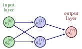
Layout of a simple neural network with two input nodes, one hidden layer with two hidden noeds and one output node
The ouput layer
Compact expressions
Output layer
Explicit derivatives
Derivatives of the hidden layer
Final expression
Completing the list
Final expressions for the biases of the hidden layer
Gradient expressions
Setting up the equations for a neural network
Layout of a neural network with three hidden layers (last layer = \( l=L=4 \), first layer \( l=0 \))
Definitions
Inputs to the activation function
Layout of input to first hidden layer \( l=1 \) from input layer \( l=0 \)
Derivatives and the chain rule
Derivative of the cost function
The back propagation equations for a neural network
Analyzing the last results
More considerations
Derivatives in terms of \( z_j^L \)
Bringing it together
Final back propagating equation
Using the chain rule and summing over all \( k \) entries
Setting up the back propagation algorithm and algorithm for a feed forward NN, initalizations
Setting up the back propagation algorithm, part 1
Setting up the back propagation algorithm, part 2
Setting up the Back propagation algorithm, part 3
Updating the gradients
Activation functions
Activation functions, Logistic and Hyperbolic ones
Relevance
Vanishing gradients
Exploding gradients
Is the Logistic activation function (Sigmoid) our choice?
Logistic function as the root of problems
The derivative of the Logistic funtion
Insights from the paper by Glorot and Bengio
The RELU function family
ELU function
Which activation function should we use?
More on activation functions, output layers
Fine-tuning neural network hyperparameters
Hidden layers
Batch Normalization
Dropout
Gradient Clipping
A top-down perspective on Neural networks
More top-down perspectives
Limitations of supervised learning with deep networks
Limitations of NNs
Homogeneous data
More limitations
Setting up a Multi-layer perceptron model for classification
Defining the cost function
Example: binary classification problem
The Softmax function
Developing a code for doing neural networks with back propagation
Collect and pre-process data
Train and test datasets
Define model and architecture
Layers
Weights and biases
Feed-forward pass
Matrix multiplications
Choose cost function and optimizer
Optimizing the cost function
Regularization
Matrix multiplication
Improving performance
Full object-oriented implementation
Evaluate model performance on test data
Adjust hyperparameters
Visualization
scikit-learn implementation
Visualization
Building neural networks in Tensorflow and Keras
Tensorflow
Using Keras
Collect and pre-process data
Building a neural network code
Learning rate methods
Usage of the above learning rate schedulers
Cost functions
Activation functions
The Neural Network
Multiclass classification
Testing the XOR gate and other gates
Layout of a simple neural network with two input nodes, one hidden layer with two hidden noeds and one output node
«
1
...
11
12
13
14
15
16
17
18
19
20
21
22
23
24
25
26
27
28
...
100
»