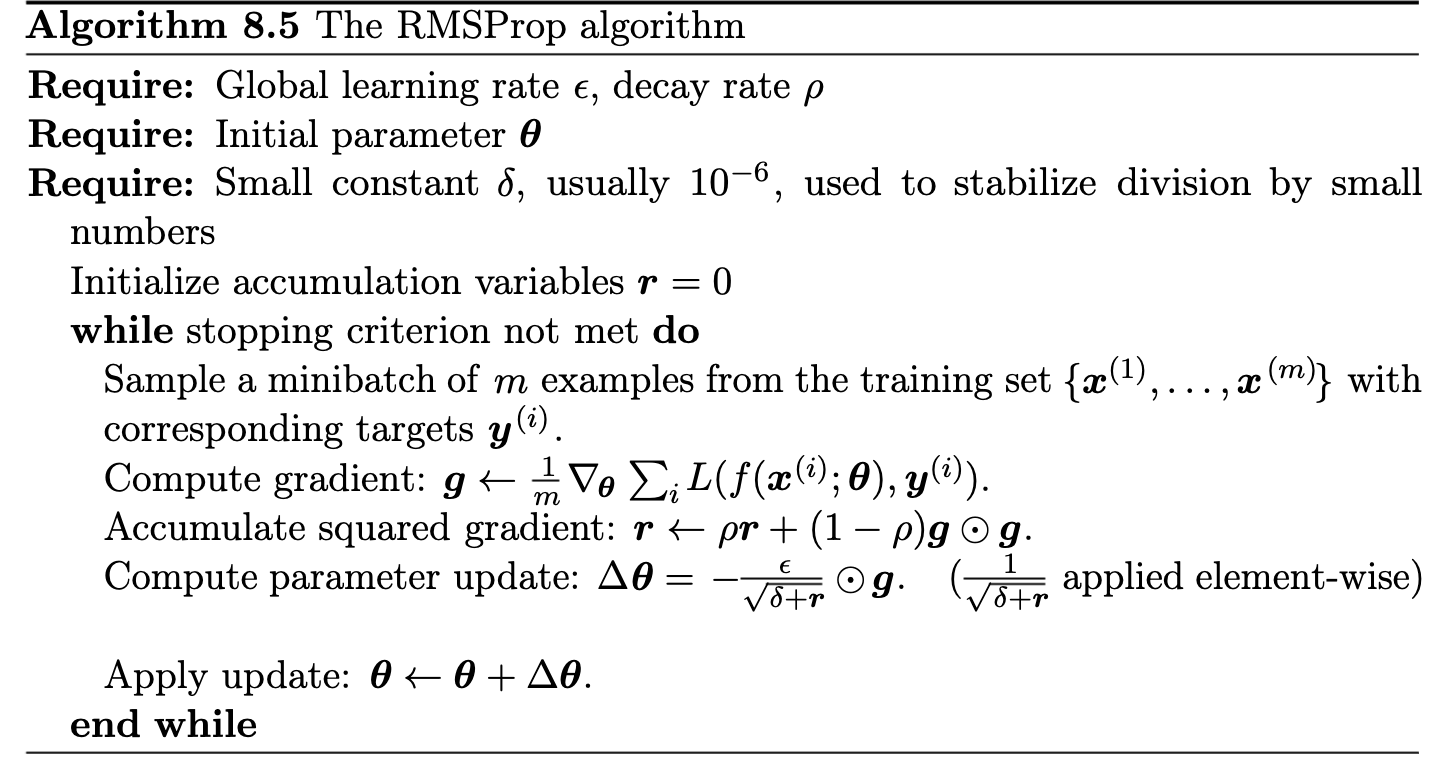
The bias-variance tradeoff

We will discuss the bias-variance tradeoff in the context of continuous predictions such as regression. However, many of the intuitions and ideas discussed here also carry over to classification tasks. Consider a dataset \( \mathcal{D} \) consisting of the data \( \mathbf{X}_\mathcal{D}=\{(y_j, \boldsymbol{x}_j), j=0\ldots n-1\} \).

Let us assume that the true data is generated from a noisy model

$$ \boldsymbol{y}=f(\boldsymbol{x}) + \boldsymbol{\epsilon} $$

where \( \epsilon \) is normally distributed with mean zero and standard deviation \( \sigma^2 \).

In our derivation of the ordinary least squares method we defined then an approximation to the function \( f \) in terms of the parameters \( \boldsymbol{\beta} \) and the design matrix \( \boldsymbol{X} \) which embody our model, that is \( \boldsymbol{\tilde{y}}=\boldsymbol{X}\boldsymbol{\beta} \).

Thereafter we found the parameters \( \boldsymbol{\beta} \) by optimizing the means squared error via the so-called cost function

$$ C(\boldsymbol{X},\boldsymbol{\beta}) =\frac{1}{n}\sum_{i=0}^{n-1}(y_i-\tilde{y}_i)^2=\mathbb{E}\left[(\boldsymbol{y}-\boldsymbol{\tilde{y}})^2\right]. $$

We can rewrite this as

$$ \mathbb{E}\left[(\boldsymbol{y}-\boldsymbol{\tilde{y}})^2\right]=\frac{1}{n}\sum_i(f_i-\mathbb{E}\left[\boldsymbol{\tilde{y}}\right])^2+\frac{1}{n}\sum_i(\tilde{y}_i-\mathbb{E}\left[\boldsymbol{\tilde{y}}\right])^2+\sigma^2. $$

The three terms represent the square of the bias of the learning method, which can be thought of as the error caused by the simplifying assumptions built into the method. The second term represents the variance of the chosen model and finally the last terms is variance of the error \( \boldsymbol{\epsilon} \).

To derive this equation, we need to recall that the variance of \( \boldsymbol{y} \) and \( \boldsymbol{\epsilon} \) are both equal to \( \sigma^2 \). The mean value of \( \boldsymbol{\epsilon} \) is by definition equal to zero. Furthermore, the function \( f \) is not a stochastics variable, idem for \( \boldsymbol{\tilde{y}} \). We use a more compact notation in terms of the expectation value

$$ \mathbb{E}\left[(\boldsymbol{y}-\boldsymbol{\tilde{y}})^2\right]=\mathbb{E}\left[(\boldsymbol{f}+\boldsymbol{\epsilon}-\boldsymbol{\tilde{y}})^2\right], $$

and adding and subtracting \( \mathbb{E}\left[\boldsymbol{\tilde{y}}\right] \) we get

$$ \mathbb{E}\left[(\boldsymbol{y}-\boldsymbol{\tilde{y}})^2\right]=\mathbb{E}\left[(\boldsymbol{f}+\boldsymbol{\epsilon}-\boldsymbol{\tilde{y}}+\mathbb{E}\left[\boldsymbol{\tilde{y}}\right]-\mathbb{E}\left[\boldsymbol{\tilde{y}}\right])^2\right], $$

which, using the abovementioned expectation values can be rewritten as

$$ \mathbb{E}\left[(\boldsymbol{y}-\boldsymbol{\tilde{y}})^2\right]=\mathbb{E}\left[(\boldsymbol{y}-\mathbb{E}\left[\boldsymbol{\tilde{y}}\right])^2\right]+\mathrm{Var}\left[\boldsymbol{\tilde{y}}\right]+\sigma^2, $$

that is the rewriting in terms of the so-called bias, the variance of the model \( \boldsymbol{\tilde{y}} \) and the variance of \( \boldsymbol{\epsilon} \).