Exercises week 34#
Coding Setup and Linear Regression#
Welcome to FYS-STK3155/4155!
In this first week will focus on getting you set up with the programs you are going to be using throughout this course. We expect that many of you will encounter some trouble with setting these programs up, as they can be extremely finnicky and prone to not working the same on all machines, so we strongly encourage you to not get discouraged, and to show up to the group-sessions where we can help you along. The group sessions are also the best place to find group partners for the projects and to be challenged on your understanding of the material, which are both essential to doing well in this course. We strongly encourage you to form groups of 2-3 participants.
If you are unable to complete this week’s exercises, don’t worry, this will likely be the most frustrating week for many of you. You have time to get back on track next week, especially if you come to the group-sessions! Note also that this week’s set of exercises does not count for the additional score. The deadline for the weekly exercises is set to Fridays, at midnight.
Learning goals#
After completing these exercises, you will know how to
Create and use a Github repository
Set up and use a virtual environment in Python
Fit an OLS model to data using scikit-learn
Fit a model on training data and evaluate it on test data
Deliverables#
Complete the following exercises while working in a jupyter notebook. Exercises 1,2 and 3 require no writing in the notebook. Then, in canvas, include
The jupyter notebook with the exercises completed
An exported PDF of the notebook (https://code.visualstudio.com/docs/datascience/jupyter-notebooks#_export-your-jupyter-notebook)
Optional: A link to your github repository, which must be set to public, include the notebook file, a README file, requirements file and gitignore file.
We require you to deliver a jupyter notebook so that we can evaluate the results of your code without needing to download and run the code of every student, as well as to teach you to use this useful tool.
Exercise 1 - Github Setup#
In this course, we require you to pay extra mind to the reproducibility of your results and the shareability of your code. The first step toward these goals is using a version control system like git and online repository like Github.
a) Download git if you don’t already have it on your machine, check with the terminal command ´git –version´ (https://git-scm.com/downloads).
b) Create a Github account(), or log in to github with your UiO account (https://github.uio.no/login).
c) Learn the basics of opening the terminal and navigating folders on your operating system. Things to learn: Opening a terminal, opening a terminal in a specific folder, listing the contents of the current folder, navigating into a folder, navigating out of a folder.
d) Download the Github CLI tool and run ´gh auth login´ in your terminal to authenticate your local machine for some of the later steps. (cli/cli). You might need to change file permissions to make it work, ask us or ChatGPT for help with these issues.
e) As an alternative to the above terminal based instructions, you could install GitHub Desktop (see https://desktop.github.com/download/) or if you prefer GitLab, GitLab desktop (see https://about.gitlab.com/install/). This sets up all communications between your PC/Laptop and the repository. This allows you to combine exercises 1 and 2 in an easy way if you don’t want to use terminarl. Keep in mind that these GUIs (graphical user interfaces) are not text editors.
Exercise 2 - Setting up a Github repository#
a) Create an empty repository for your coursework in this course in your browser at github.com (or uio github).
b) Open a terminal in the location you want to create your local folder for this repository, like your desktop.
c) Clone the repository to your laptop using the terminal command ´gh repo clone username/repository-name´. This creates a folder with the same name as the repository. Moving it or renaming it might require some extra steps.
d) Download this jupyter notebook. Add the notebook to the local folder.
e) Run the ´git add .´ command command in a terminal opened in the local folder to stage the current changes in the folder to be commited to the version control history. Run ´git status´ to see the staged files.
f) Run the ´git commit -m “Adding first weekly assignment file”´ command to commit the staged changes to the version control history. Run ´git status´ to see that no files are staged.
g) Run the ´git push” command to upload the commited changes to the remote repository on Github.
h) Add a file called README.txt to the repository at Github.com. Don’t do this in your local folder. Add a suitable title for your repository and some inforomation to the file.
i) Run the ´git fetch origin´ command to fetch the latest remote changes to your repository.
j) Run the ´git pull´ command to download and update files to match the remote changes.
Exercise 3 - Setting up a Python virtual environment#
Following the themes from the previous exercises, another way of improving the reproducibility of your results and shareability of your code is having a good handle on which python packages you are using.
There are many ways to manage your packages in Python, and you are free to use any approach you want, but in this course we encourage you to use something called a virtual environment. A virtual environemnt is a folder in your project which contains a Python runtime executable as well as all the packages you are using in the current project. In this way, each of your projects has its required set of packages installed in the same folder, so that if anything goes wrong while managing your packages it only affects the one project, and if multiple projects require different versions of the same package, you don’t need to worry about messing up old projects. Also, it’s easy to just delete the folder and start over if anything goes wrong.
Virtual environments are typically created, activated, managed and updated using terminal commands, but for now we recommend that you let for example VS Code (a popular cross-paltform package) handle it for you to make the coding experience much easier. If you are familiar with another approach for virtual environments that works for you, feel free to keep doing it that way.
a) Open this notebook in VS Code (https://code.visualstudio.com/Download). Download the Python and Jupyter extensions.
b) Press ´Cmd + Shift + P´, then search and run ´Python: Create Environment…´
c) Select ´Venv´
d) Choose the most up-to-date version of Python your have installed.
e) Press ´Cmd + Shift + P´, then search and run ´Python: Select Interpreter´
f) Selevet the (.venv) option you just created.
g) Open a terminal in VS Code, the venv name should be visible at the beginning of the line. Run pip list to see that there are no packages install in the environment.
h) In this terminal, run pip install matplotlib numpy scikit-learn. This will install the listed packages.
i) To make these installations reproducible, which is important for reproducing results and sharing your code, run ´pip freeze > requirements.txt´ to create the file requirements.txt with all your dependencies.
Now, anyone who wants to recreate your package setup can download your requirements.txt file and run ´pip install -r requirements.txt´ to install the correct packages and versions. To keep the requirements.txt file up to date with your environment, you will need to re-run the freeze command whenever you install a new package.
j) Create a .gitignore file at the root of your project folder, and add the line ´.venv´ to it. This way, you won’t try to upload a copy of all your python packages when you regularly push your changes to Github. Ignored files should not show up when you run ´git status´, and are not staged when running ´git add .´, try it!
Exercise 3 - Fitting an OLS model to data#
Great job on getting through all of that! Now it is time to do some actual machine learning!
a) Complete the code below so that you fit a second order polynomial to the data. You will need to look up some scikit-learn documentation online (look at the imported functions for hints).
b) Compute the mean square error for the line model and for the second degree polynomial model.
import numpy as np
import matplotlib.pyplot as plt
from sklearn.preprocessing import PolynomialFeatures # use the fit_transform method of the created object!
from sklearn.linear_model import LinearRegression
from sklearn.metrics import mean_squared_error
n = 100
x = np.random.rand(n, 1)
y = 2.0 + 5 * x**2 + 0.1 * np.random.randn(n, 1)
line_model = LinearRegression().fit(x, y)
line_predict = line_model.predict(x)
#line_mse = ...
#poly_features = ...
#poly_model = LinearRegression().fit(..., y)
#poly_predict = ...
#poly_mse = ...
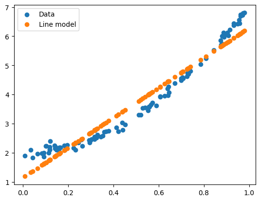
plt.scatter(x, y, label = "Data")
plt.scatter(x, line_predict, label = "Line model")
plt.legend()
plt.show()
Exercise 4 - The train-test split#
Hopefully your model fit the data quite well, but to know how well the model actually generalizes to unseen data, which is most often what we care about, we need to split our data into training and testing data.
from sklearn.model_selection import train_test_split
a) Complete the code below so that the polynomial features and the targets y get split into training and test data.
b) What is the shape of X_test?
c) Fit your model to X_train
d) Compute the MSE when your model predicts on the training data and on the testing data, using y_train and y_test as targets for the two cases.
e) Why do we not fit the model to X_test?
polynomial_features = ...

#X_train, X_test, y_train, y_test = train_test_split(polynomial_features, y, test_size=0.2)