Exercises week 36#
Deriving and Implementing Ridge Regression#
Learning goals#
After completing these exercises, you will know how to
Take more derivatives of simple products between vectors and matrices
Implement Ridge regression using the analytical expressions
Scale data appropriately for linear regression
Evaluate a model across two different hyperparameters
Exercise 1 - Choice of model and degrees of freedom#
a) How many degrees of freedom does an OLS model fit to the features \(x, x^2, x^3\) and the intercept have?
b) Why is it bad for a model to have too many degrees of freedom?
c) Why is it bad for a model to have too few degrees of freedom?
d) Read chapter 3.4.1 of Hastie et al.’s book. What is the expression for the effective degrees of freedom of the ridge regression fit?
e) Why might we want to use Ridge regression instead of OLS?
f) Why migth we want to use OLS instead of Ridge regression?
Exercise 2 - Deriving the expression for Ridge Regression#
The aim here is to derive the expression for the optimal parameters using Ridge regression.
The expression for the standard Mean Squared Error (MSE) which we used to define our cost function and the equations for the ordinary least squares (OLS) method, was given by the optimization problem
By minimizing the above equation with respect to the parameters \(\boldsymbol{\beta}\) we could then obtain an analytical expression for the parameters \(\boldsymbol{\hat\beta_{OLS}}\).
We can add a regularization parameter \(\lambda\) by defining a new cost function to be optimized, that is
which leads to the Ridge regression minimization problem. (One can require as part of the optimization problem that \(\vert\vert \boldsymbol{\beta}\vert\vert_2^2\le t\), where \(t\) is a finite number larger than zero. We will not implement that in this course.)
a) Expression for Ridge regression#
Show that the optimal parameters
with \(\boldsymbol{I}\) being a \(p\times p\) identity matrix.
The ordinary least squares result is
Exercise 3 - Scaling data#
import numpy as np
import matplotlib.pyplot as plt
from sklearn.model_selection import train_test_split
from sklearn.preprocessing import StandardScaler
n = 100
x = np.linspace(-3, 3, n)
y = np.exp(-x**2) + 1.5 * np.exp(-(x-2)**2) + np.random.normal(n)
a) Adapt your function from last week to only include the intercept column if the boolean argument intercept is set to true.
def polynomial_features(x, p, intercept=False):
    n = len(x)
    X = np.zeros((n, p + 1))
    #X[:, 0] = ...
    #X[:, 1] = ...
    #X[:, 2] = ...
    # could this be a loop?
def polynomial_features(x, p, intercept=False):
    n = len(x)
    X = np.zeros((n, p))
    X[:, 0] = x[:]
    X[:, 1] = x**2
    X[:, 2] = x**3
    return X
b) Split your data into training and test data(80/20 split)
X = polynomial_features(x, 3)
X_train, X_test, y_train, y_test = train_test_split(X, y, test_size=0.2)
x_train = X_train[:, 0] # These are used for plotting
x_test = X_test[:, 0] # These are used for plotting
c) Scale your design matrix with the sklearn standard scaler, though based on the mean and standard deviation of the training data only.
scaler = StandardScaler()
scaler.fit(X_train)
X_train_s = scaler.transform(X_train)
X_test_s = scaler.transform(X_test)
y_offset = np.mean(y_train)
Exercise 4 - Implementing Ridge Regression#
a) Implement a function for computing the optimal Ridge parameters using the expression from 2a).
def Ridge_parameters(X, y):
    # Assumes X is scaled and has no intercept column
    return np.linalg.inv(X.T @ X) @ X.T @ y

beta = Ridge_parameters(X_train_s, y_train)
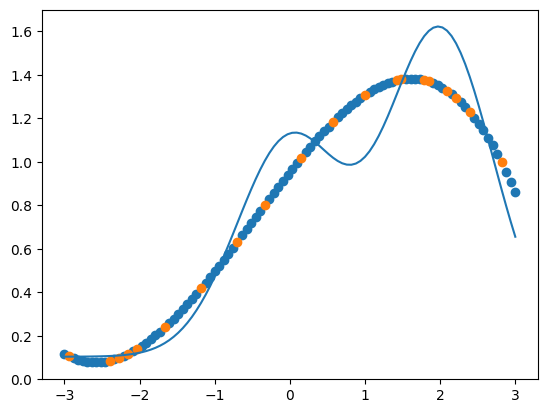
b) Fit a model to the data, and plot the prediction using both the training and test x-values extracted before scaling, and the y_offset.
plt.plot(x, y)
plt.scatter(x_train, X_train_s @ beta + y_offset)
plt.scatter(x_test, X_test_s @ beta + y_offset)
<matplotlib.collections.PathCollection at 0x113e21950>
Exercise 4 - Testing multiple hyperparameters#
a) Compute the MSE of your ridge model for polynomials of degrees 1 to 5 with lambda set to 0.01. Plot the MSE as a function of polynomial degree.
b) Compute the MSE of your ridge model for a polynomial with degree 3, and with lambdas from \(10^{-1}\) to \(10^{-5}\) on a logarithmic scale. Plot the MSE as a function of lambda.
c) Compute the MSE of your ridge model for polynomials of degrees 1 to 5, and with lambdas from \(10^{-1}\) to \(10^{-5}\) on a logarithmic scale. Plot the MSE as a function of polynomial degree and lambda using a heatmap.