Week 35: From Ordinary Linear Regression to Ridge and Lasso Regression#
Morten Hjorth-Jensen, Department of Physics, University of Oslo
Date: August 25-29, 2025
Plans for week 35#
The main topics are:
Brief repetition from last week
Discussions of the equations for ordinary least squares (OLS)
Discussion on how to prepare data and examples of applications of linear regression
Mathematical interpretations of OLS
Introduction of Ridge and Lasso regression
Reading recommendations:#
These lecture notes
Video of lecture at https://youtu.be/2mvizAQFST8
Whiteboard notes at CompPhysics/MachineLearning
Goodfellow, Bengio and Courville, Deep Learning, chapter 2 on linear algebra
Raschka et al on preprocessing of data, relevant for exercise 3 this week, see chapter 4.
For exercise 1 of week 35, the book by A. Aldo Faisal, Cheng Soon Ong, and Marc Peter Deisenroth on the Mathematics of Machine Learning, may be very relevant. In particular chapter 5 at URL”https://mml-book.github.io/” (section 5.5 on derivatives) is very useful for exercise 1 this coming week.
Reminder from last week#
We need first a reminder from last week about linear regression. We are going to fit a continuous function with linear parameterization in terms of the parameters \(\boldsymbol{\theta}\) and our first encounter is ordinary least squares.
It is the method of choice for fitting a continuous function
Gives an excellent introduction to central Machine Learning features with understandable pedagogical links to other methods like Neural Networks, Support Vector Machines etc
Analytical expression for the fitting parameters \(\boldsymbol{\theta}\)
Analytical expressions for statistical propertiers like mean values, variances, confidence intervals and more
Analytical relation with probabilistic interpretations
Easy to introduce basic concepts like bias-variance tradeoff, cross-validation, resampling and regularization techniques and many other ML topics
Easy to code! And links well with classification problems and logistic regression and neural networks
Allows for easy hands-on understanding of gradient descent methods
and many more features
For more discussions of Ridge and Lasso regression, Wessel van Wieringen’s article is highly recommended. Similarly, Mehta et al’s article is also recommended.
The equations for ordinary least squares#
Our data which we want to apply a machine learning method on, consist of a set of inputs \(\boldsymbol{x}^T=[x_0,x_1,x_2,\dots,x_{n-1}]\) and the outputs we want to model \(\boldsymbol{y}^T=[y_0,y_1,y_2,\dots,y_{n-1}]\). We assume that the output data can be represented (for a regression case) by a continuous function \(f\) through
or in general
where \(\boldsymbol{\epsilon}\) represents some noise which is normally assumed to be distributed via a normal probability distribution with zero mean value and a variance \(\sigma^2\).
In linear regression we approximate the unknown function with another continuous function \(\tilde{\boldsymbol{y}}(\boldsymbol{x})\) which depends linearly on some unknown parameters \(\boldsymbol{\theta}^T=[\theta_0,\theta_1,\theta_2,\dots,\theta_{p-1}]\).
Last week we introduced the so-called design matrix in order to define the approximation \(\boldsymbol{\tilde{y}}\) via the unknown quantity \(\boldsymbol{\theta}\) as
and in order to find the optimal parameters \(\theta_i\) we defined a function which gives a measure of the spread between the values \(y_i\) (which represent the output values we want to reproduce) and the parametrized values \(\tilde{y}_i\), namely the so-called cost/loss function.
The cost/loss function#
We used the mean squared error to define the way we measure the quality of our model
or using the matrix \(\boldsymbol{X}\) and in a more compact matrix-vector notation as
This function represents one of many possible ways to define the so-called cost function.
It is also common to define the function \(C\) as
since when taking the first derivative with respect to the unknown parameters \(\theta\), the factor of \(2\) cancels out.
Interpretations and optimizing our parameters#
The function
can be linked to the variance of the quantity \(y_i\) if we interpret the latter as the mean value. When linking (see the discussions next week) with the maximum likelihood approach below, we will indeed interpret \(y_i\) as a mean value
where \(\langle y_i \rangle\) is the mean value. Keep in mind also that till now we have treated \(y_i\) as the exact value. Normally, the output (response, target, dependent or outcome) variable \(y_i\) is the outcome of a numerical experiment or another type of experiment and could thus be treated itself as an approximation to the true value. It is then always accompanied by an error estimate, often limited to a statistical error estimate given by the standard deviation discussed earlier. In the discussion here we will treat \(y_i\) as our exact value for the output variable.
In order to find the parameters \(\theta_i\) we will then minimize the spread of \(C(\boldsymbol{\theta})\), that is we are going to solve the problem
In practical terms it means we will require
which results in
or in a matrix-vector form as (multiplying away the factor \(-2/n\), see derivation below)
Interpretations and optimizing our parameters#
We can rewrite, see the derivations below,
as
and if the matrix \(\boldsymbol{X}^T\boldsymbol{X}\) is invertible we have the solution
We note also that since our design matrix is defined as \(\boldsymbol{X}\in {\mathbb{R}}^{n\times p}\), the product \(\boldsymbol{X}^T\boldsymbol{X} \in {\mathbb{R}}^{p\times p}\). In most cases we have that \(p \ll n\). In our example case below we have \(p=5\) meaning. We end up with inverting a small \(5\times 5\) matrix. This is a rather common situation, in many cases we end up with low-dimensional matrices to invert. The methods discussed here and for many other supervised learning algorithms like classification with logistic regression or support vector machines, exhibit dimensionalities which allow for the usage of direct linear algebra methods such as LU decomposition or Singular Value Decomposition (SVD) for finding the inverse of the matrix \(\boldsymbol{X}^T\boldsymbol{X}\).
Small question: When inverting the matrix $\boldsymbol{X}^T\boldsymbol{X}, what kind of problems can we expect?
Some useful matrix and vector expressions#
The following matrix and vector relation will be useful here and for the rest of the course. Vectors are always written as boldfaced lower case letters and matrices as upper case boldfaced letters. In the following we will discuss how to calculate derivatives of various matrices relevant for machine learning. We will often represent our data in terms of matrices and vectors.
Let us introduce first some conventions. We assume that \(\boldsymbol{y}\) is a vector of length \(m\), that is it has \(m\) elements \(y_0,y_1,\dots, y_{m-1}\). By convention we start labeling vectors with the zeroth element, as are arrays in Python and C++/C, for example. Similarly, we have a vector \(\boldsymbol{x}\) of length \(n\), that is \(\boldsymbol{x}^T=[x_0,x_1,\dots, x_{n-1}]\).
We assume also that \(\boldsymbol{y}\) is a function of \(\boldsymbol{x}\) through some given function \(f\)
The Jacobian#
We define the partial derivatives of the various components of \(\boldsymbol{y}\) as functions of \(x_i\) in terms of the so-called Jacobian matrix
which is an \(m\times n\) matrix. If \(\boldsymbol{x}\) is a scalar, then the Jacobian is only a single-column vector, or an \(m\times 1\) matrix. If on the other hand \(\boldsymbol{y}\) is a scalar, the Jacobian becomes a \(1\times n\) matrix.
When this matrix is a square matrix \(m=n\), its determinant is often referred to as the Jacobian determinant. Both the matrix and (if \(m=n\)) the determinant are often referred to simply as the Jacobian. The Jacobian matrix represents the differential of \(\boldsymbol{y}\) at every point where the vector is differentiable.
Derivatives, example 1#
Let now \(\boldsymbol{y}=\boldsymbol{A}\boldsymbol{x}\), where \(\boldsymbol{A}\) is an \(m\times n\) matrix and the matrix does not depend on \(\boldsymbol{x}\). If we write out the vector \(\boldsymbol{y}\) compoment by component we have
with \(\forall i=0,1,2,\dots,m-1\). The individual matrix elements of \(\boldsymbol{A}\) are given by the symbol \(a_{ij}\). It follows that the partial derivatives of \(y_i\) with respect to \(x_k\)
From this we have, using the definition of the Jacobian
Example 2#
We define a scalar (our cost/loss functions are in general also scalars, just think of the mean squared error) as the result of some matrix vector multiplications
with \(\boldsymbol{y}\) a vector of length \(m\), \(\boldsymbol{A}\) an \(m\times n\) matrix and \(\boldsymbol{x}\) a vector of length \(n\). We assume also that \(\boldsymbol{A}\) does not depend on any of the two vectors. In order to find the derivative of \(\alpha\) with respect to the two vectors, we define an intermediate vector \(\boldsymbol{z}\). We define first \(\boldsymbol{z}^T=\boldsymbol{y}^T\boldsymbol{A}\), a vector of length \(n\). We have then, using the definition of the Jacobian,
which means that (using our previous example and keeping track of our definition of the derivative of a scalar) we have
Note that the resulting vector elements are the same for \(\boldsymbol{z}^T\) and \(\boldsymbol{z}\), the only difference is that one is just the transpose of the other. We have the transposed here since we have used that the inner product of two vectors is a scalar.
Since \(\alpha\) is a scalar we have \(\alpha =\alpha^T=\boldsymbol{x}^T\boldsymbol{A}^T\boldsymbol{y}\). Defining now \(\boldsymbol{z}^T=\boldsymbol{x}^T\boldsymbol{A}^T\) we find that
Example 3#
We start with a new scalar but where now the vector \(\boldsymbol{y}\) is replaced by a vector \(\boldsymbol{x}\) and the matrix \(\boldsymbol{A}\) is a square matrix with dimension \(n\times n\).
with \(\boldsymbol{x}\) a vector of length \(n\).
We write out the specific sums involved in the calculation of \(\alpha\)
taking the derivative of \(\alpha\) with respect to a given component \(x_k\) we get the two sums
for \(\forall k =0,1,2,\dots,n-1\). We identify these sums as
If the matrix \(\boldsymbol{A}\) is symmetric, that is \(\boldsymbol{A}=\boldsymbol{A}^T\), we have
Example 4#
We let the scalar \(\alpha\) be defined by
where both \(\boldsymbol{y}\) and \(\boldsymbol{x}\) have the same length \(n\), or if we wish to think of them as column vectors, they have dimensions \(n\times 1\). We assume that both \(\boldsymbol{y}\) and \(\boldsymbol{x}\) depend on a vector \(\boldsymbol{z}\) of the same length. To calculate the derivative of \(\alpha\) with respect to a given component \(z_k\) we need first to write out the inner product that defines \(\alpha\) as
and the partial derivative
for \(\forall k =0,1,2,\dots,n-1\). We can rewrite the partial derivative in a more compact form as
and if \(\boldsymbol{y}=\boldsymbol{x}\) we have
The mean squared error and its derivative#
We defined earlier a possible cost function using the mean squared error
or using the design/feature matrix \(\boldsymbol{X}\) we have the more compact matrix-vector
We note that the design matrix \(\boldsymbol{X}\) does not depend on the unknown parameters defined by the vector \(\boldsymbol{\theta}\). We are now interested in minimizing the cost function with respect to the unknown parameters \(\boldsymbol{\theta}\).
The mean squared error is a scalar and if we use the results from example three above, we can define a new vector
which depends on \(\boldsymbol{\theta}\). We rewrite the cost function as
with partial derivative
and using that
where we used the result from example two above. Inserting the last expression we obtain
or as
Meet the Hessian Matrix#
A very important matrix we will meet again and again in machine learning is the Hessian. It is given by the second derivative of the cost function with respect to the parameters \(\boldsymbol{\theta}\). Using the above expression for derivatives of vectors and matrices, we find that the second derivative of the mean squared error as cost function is,
The Hessian matrix plays an important role and is defined here as
For ordinary least squares, it is inversely proportional (derivation next week) with the variance of the optimal parameters \(\hat{\boldsymbol{\theta}}\). Furthermore, we will see next week that it is (aside the factor \(1/n\)) equal to the covariance matrix. It plays also a very important role in optmization algorithms and Principal Component Analysis as a way to reduce the dimensionality of a machine learning/data analysis problem. We will discuss this in greater detail next week when we introduce gradient methods.
Linear algebra question: Can we use the Hessian matrix to say something about properties of the cost function (our optmization problem)? (hint: think about convex or concave problems and how to relate these to a matrix!).
Interpretations and optimizing our parameters#
The residuals \(\boldsymbol{\epsilon}\) are in turn given by
and with
we have
meaning that the solution for \(\boldsymbol{\theta}\) is the one which minimizes the residuals.
Example relevant for the exercises#
In order to understand the relation among the predictors \(p\), the set of data \(n\) and the target (outcome, output etc) \(\boldsymbol{y}\), we condiser a simple polynomial fit. We assume our data can represented by a fourth-order polynomial. For the \(i\)th component we have
we have five predictors/features. The first is the intercept \(\theta_0\). The other terms are \(\theta_i\) with \(i=1,2,3,4\). Furthermore we have \(n\) entries for each predictor. It means that our design matrix is an \(n\times p\) matrix \(\boldsymbol{X}\).
Own code for Ordinary Least Squares#
It is rather straightforward to implement the matrix inversion and obtain the parameters \(\boldsymbol{\theta}\). After having defined the matrix \(\boldsymbol{X}\) and the outputs \(\boldsymbol{y}\) we have
# matrix inversion to find theta
# First we set up the data
import numpy as np
x = np.random.rand(100)
y = 2.0+5*x*x+0.1*np.random.randn(100)
# and then the design matrix X including the intercept
#  The design matrix now as function of a fourth-order polynomial
X = np.zeros((len(x),5))
X[:,0] = 1.0
X[:,1] = x
X[:,2] = x**2
X[:,3] = x**3
X[:,4] = x**4
theta = (np.linalg.inv(X.T @ X) @ X.T ) @ y
# and then make the prediction
ytilde = X @ theta
Alternatively, you can use the least squares functionality in Numpy as
fit = np.linalg.lstsq(X, y, rcond =None)[0]
ytildenp = np.dot(fit,X.T)
Adding error analysis and training set up#
We can easily test our fit by computing the \(R2\) score that we discussed in connection with the functionality of Scikit-Learn in the introductory slides. Since we are not using Scikit-Learn here we can define our own \(R2\) function as
def R2(y_data, y_model):
    return 1 - np.sum((y_data - y_model) ** 2) / np.sum((y_data - np.mean(y_data)) ** 2)
and we would be using it as
print(R2(y,ytilde))
We can easily add our MSE score as
def MSE(y_data,y_model):
    n = np.size(y_model)
    return np.sum((y_data-y_model)**2)/n

print(MSE(y,ytilde))
and finally the relative error as
def RelativeError(y_data,y_model):
    return abs((y_data-y_model)/y_data)
print(RelativeError(y, ytilde))
Splitting our Data in Training and Test data#
It is normal in essentially all Machine Learning studies to split the data in a training set and a test set (sometimes also an additional validation set). Scikit-Learn has an own function for this. There is no explicit recipe for how much data should be included as training data and say test data. An accepted rule of thumb is to use approximately \(2/3\) to \(4/5\) of the data as training data. We will postpone a discussion of this splitting to the end of these notes and our discussion of the so-called bias-variance tradeoff. Here we limit ourselves to repeat the above equation of state fitting example but now splitting the data into a training set and a test set.
The complete code with a simple data set#
%matplotlib inline

import os
import numpy as np
import pandas as pd
import matplotlib.pyplot as plt
from sklearn.model_selection import train_test_split


def R2(y_data, y_model):
    return 1 - np.sum((y_data - y_model) ** 2) / np.sum((y_data - np.mean(y_data)) ** 2)
def MSE(y_data,y_model):
    n = np.size(y_model)
    return np.sum((y_data-y_model)**2)/n

x = np.random.rand(100)
y = 2.0+5*x*x+0.1*np.random.randn(100)


#  The design matrix now as function of a fourth-order polynomial
X = np.zeros((len(x),5))
X[:,0] = 1.0
X[:,1] = x
X[:,2] = x**2
X[:,3] = x**3
X[:,4] = x**4
# We split the data in test and training data
X_train, X_test, y_train, y_test = train_test_split(X, y, test_size=0.2)
# matrix inversion to find theta
theta = np.linalg.inv(X_train.T @ X_train) @ X_train.T @ y_train
print(theta)
# and then make the prediction
ytilde = X_train @ theta
print("Training R2")
print(R2(y_train,ytilde))
print("Training MSE")
print(MSE(y_train,ytilde))
ypredict = X_test @ theta
print("Test R2")
print(R2(y_test,ypredict))
print("Test MSE")
print(MSE(y_test,ypredict))
Making your own test-train splitting#
# equivalently in numpy
def train_test_split_numpy(inputs, labels, train_size, test_size):
    n_inputs = len(inputs)
    inputs_shuffled = inputs.copy()
    labels_shuffled = labels.copy()

    np.random.shuffle(inputs_shuffled)
    np.random.shuffle(labels_shuffled)

    train_end = int(n_inputs*train_size)
    X_train, X_test = inputs_shuffled[:train_end], inputs_shuffled[train_end:]
    Y_train, Y_test = labels_shuffled[:train_end], labels_shuffled[train_end:]

    return X_train, X_test, Y_train, Y_test
But since scikit-learn has its own function for doing this and since it interfaces easily with tensorflow and other libraries, we normally recommend using the latter functionality.
Reducing the number of degrees of freedom, overarching view#
Many Machine Learning problems involve thousands or even millions of features for each training instance. Not only does this make training extremely slow, it can also make it much harder to find a good solution, as we will see. This problem is often referred to as the curse of dimensionality. Fortunately, in real-world problems, it is often possible to reduce the number of features considerably, turning an intractable problem into a tractable one.
Later we will discuss some of the most popular dimensionality reduction techniques: the principal component analysis (PCA), Kernel PCA, and Locally Linear Embedding (LLE).
Principal component analysis and its various variants deal with the problem of fitting a low-dimensional affine subspace to a set of of data points in a high-dimensional space. With its family of methods it is one of the most used tools in data modeling, compression and visualization.
Preprocessing our data#
Before we proceed however, we will discuss how to preprocess our data. Till now and in connection with our previous examples we have not met so many cases where we are too sensitive to the scaling of our data. Normally the data may need a rescaling and/or may be sensitive to extreme values. Scaling the data renders our inputs much more suitable for the algorithms we want to employ.
For data sets gathered for real world applications, it is rather normal that different features have very different units and numerical scales. For example, a data set detailing health habits may include features such as age in the range \(0-80\), and caloric intake of order \(2000\). Many machine learning methods sensitive to the scales of the features and may perform poorly if they are very different scales. Therefore, it is typical to scale the features in a way to avoid such outlier values.
Functionality in Scikit-Learn#
Scikit-Learn has several functions which allow us to rescale the data, normally resulting in much better results in terms of various accuracy scores. The StandardScaler function in Scikit-Learn ensures that for each feature/predictor we study the mean value is zero and the variance is one (every column in the design/feature matrix). This scaling has the drawback that it does not ensure that we have a particular maximum or minimum in our data set. Another function included in Scikit-Learn is the MinMaxScaler which ensures that all features are exactly between \(0\) and \(1\). The
More preprocessing#
The Normalizer scales each data point such that the feature vector has a euclidean length of one. In other words, it projects a data point on the circle (or sphere in the case of higher dimensions) with a radius of 1. This means every data point is scaled by a different number (by the inverse of it’s length). This normalization is often used when only the direction (or angle) of the data matters, not the length of the feature vector.
The RobustScaler works similarly to the StandardScaler in that it ensures statistical properties for each feature that guarantee that they are on the same scale. However, the RobustScaler uses the median and quartiles, instead of mean and variance. This makes the RobustScaler ignore data points that are very different from the rest (like measurement errors). These odd data points are also called outliers, and might often lead to trouble for other scaling techniques.
Frequently used scaling functions#
Many features are often scaled using standardization to improve performance. In Scikit-Learn this is given by the StandardScaler function as discussed above. It is easy however to write your own. Mathematically, this involves subtracting the mean and divide by the standard deviation over the data set, for each feature:
where \(\overline{x}_j\) and \(\sigma(x_j)\) are the mean and standard deviation, respectively, of the feature \(x_j\). This ensures that each feature has zero mean and unit standard deviation. For data sets where we do not have the standard deviation or don’t wish to calculate it, it is then common to simply set it to one.
Example of own Standard scaling#
Let us consider the following vanilla example where we use both Scikit-Learn and write our own function as well. We produce a simple test design matrix with random numbers. Each column could then represent a specific feature whose mean value is subracted.
import sklearn.linear_model as skl
from sklearn.metrics import mean_squared_error
from sklearn.model_selection import  train_test_split
from sklearn.preprocessing import MinMaxScaler, StandardScaler, Normalizer
import numpy as np
import pandas as pd
from IPython.display import display
np.random.seed(100)
# setting up a 10 x 5 matrix
rows = 10
cols = 5
X = np.random.randn(rows,cols)
XPandas = pd.DataFrame(X)
display(XPandas)
print(XPandas.mean())
print(XPandas.std())
XPandas = (XPandas -XPandas.mean())
display(XPandas)
#  This option does not include the standard deviation
scaler = StandardScaler(with_std=False)
scaler.fit(X)
Xscaled = scaler.transform(X)
display(XPandas-Xscaled)
Small exercise: perform the standard scaling by including the standard deviation and compare with what Scikit-Learn gives.
Min-Max Scaling#
Another commonly used scaling method is min-max scaling. This is very useful for when we want the features to lie in a certain interval. To scale the feature \(x_j\) to the interval \([a, b]\), we can apply the transformation
where \(\min(x_j)\) and \(\max(x_j)\) return the minimum and maximum value of \(x_j\) over the data set, respectively.
Testing the Means Squared Error as function of Complexity#
One of the aims is to reproduce Figure 2.11 of Hastie et al.
Our data is defined by \(x\in [-3,3]\) with a total of for example \(100\) data points.
np.random.seed()
n = 100
maxdegree = 14
# Make data set.
x = np.linspace(-3, 3, n).reshape(-1, 1)
y = np.exp(-x**2) + 1.5 * np.exp(-(x-2)**2)+ np.random.normal(0, 0.1, x.shape)
where \(y\) is the function we want to fit with a given polynomial.
Write a first code which sets up a design matrix \(X\) defined by a fourth-order polynomial. Scale your data and split it in training and test data.
import matplotlib.pyplot as plt
import numpy as np
from sklearn.linear_model import LinearRegression
from sklearn.preprocessing import PolynomialFeatures
from sklearn.model_selection import train_test_split
from sklearn.pipeline import make_pipeline


np.random.seed(2018)
n = 50
maxdegree = 5
# Make data set.
x = np.linspace(-3, 3, n).reshape(-1, 1)
y = np.exp(-x**2) + 1.5 * np.exp(-(x-2)**2)+ np.random.normal(0, 0.1, x.shape)
TestError = np.zeros(maxdegree)
TrainError = np.zeros(maxdegree)
polydegree = np.zeros(maxdegree)
x_train, x_test, y_train, y_test = train_test_split(x, y, test_size=0.2)
scaler = StandardScaler()
scaler.fit(x_train)
x_train_scaled = scaler.transform(x_train)
x_test_scaled = scaler.transform(x_test)

for degree in range(maxdegree):
    model = make_pipeline(PolynomialFeatures(degree=degree), LinearRegression(fit_intercept=False))
    clf = model.fit(x_train_scaled,y_train)
    y_fit = clf.predict(x_train_scaled)
    y_pred = clf.predict(x_test_scaled)
    polydegree[degree] = degree
    TestError[degree] = np.mean( np.mean((y_test - y_pred)**2) )
    TrainError[degree] = np.mean( np.mean((y_train - y_fit)**2) )

plt.plot(polydegree, TestError, label='Test Error')
plt.plot(polydegree, TrainError, label='Train Error')
plt.legend()
plt.show()
Mathematical Interpretation of Ordinary Least Squares#
What is presented here is a mathematical analysis of various regression algorithms (ordinary least squares, Ridge and Lasso Regression). The analysis is based on an important algorithm in linear algebra, the so-called Singular Value Decomposition (SVD).
We have shown that in ordinary least squares the optimal parameters \(\theta\) are given by
The hat over \(\boldsymbol{\theta}\) means we have the optimal parameters after minimization of the cost function.
This means that our best model is defined as
We now define a matrix
We can rewrite
The matrix \(\boldsymbol{A}\) has the important property that \(\boldsymbol{A}^2=\boldsymbol{A}\). This is the definition of a projection matrix. We can then interpret our optimal model \(\tilde{\boldsymbol{y}}\) as being represented by an orthogonal projection of \(\boldsymbol{y}\) onto a space defined by the column vectors of \(\boldsymbol{X}\). In our case here the matrix \(\boldsymbol{A}\) is a square matrix. If it is a general rectangular matrix we have an oblique projection matrix.
Residual Error#
We have defined the residual error as
The residual errors are then the projections of \(\boldsymbol{y}\) onto the orthogonal component of the space defined by the column vectors of \(\boldsymbol{X}\).
Simple case#
If the matrix \(\boldsymbol{X}\) is an orthogonal (or unitary in case of complex values) matrix, we have
In this case the matrix \(\boldsymbol{A}\) becomes
and we have the obvious case
This serves also as a useful test of our codes.
The singular value decomposition#
The examples we have looked at so far are cases where we normally can invert the matrix \(\boldsymbol{X}^T\boldsymbol{X}\). Using a polynomial expansion where we fit of various functions leads to row vectors of the design matrix which are essentially orthogonal due to the polynomial character of our model. Obtaining the inverse of the design matrix is then often done via a so-called LU, QR or Cholesky decomposition.
As we will also see in the first project, this may however not the be case in general and a standard matrix inversion algorithm based on say LU, QR or Cholesky decomposition may lead to singularities. We will see examples of this below and in other examples.
There is however a way to circumvent this problem and also gain some insights about the ordinary least squares approach, and later shrinkage methods like Ridge and Lasso regressions.
This is given by the Singular Value Decomposition (SVD) algorithm, perhaps the most powerful linear algebra algorithm. The SVD provides a numerically stable matrix decomposition that is used in a large swath oc applications and the decomposition is always stable numerically.
In machine learning it plays a central role in dealing with for example design matrices that may be near singular or singular. Furthermore, as we will see here, the singular values can be related to the covariance matrix (and thereby the correlation matrix) and in turn the variance of a given quantity. It plays also an important role in the principal component analysis where high-dimensional data can be reduced to the statistically relevant features.
Linear Regression Problems#
One of the typical problems we encounter with linear regression, in particular
when the matrix \(\boldsymbol{X}\) (our so-called design matrix) is high-dimensional,
are problems with near singular or singular matrices. The column vectors of \(\boldsymbol{X}\)
may be linearly dependent, normally referred to as super-collinearity.
This means that the matrix may be rank deficient and it is basically impossible to
to model the data using linear regression. As an example, consider the matrix
The columns of \(\boldsymbol{X}\) are linearly dependent. We see this easily since the the first column is the row-wise sum of the other two columns. The rank (more correct, the column rank) of a matrix is the dimension of the space spanned by the column vectors. Hence, the rank of \(\mathbf{X}\) is equal to the number of linearly independent columns. In this particular case the matrix has rank 2.
Super-collinearity of an \((n \times p)\)-dimensional design matrix \(\mathbf{X}\) implies that the inverse of the matrix \(\boldsymbol{X}^T\boldsymbol{X}\) (the matrix we need to invert to solve the linear regression equations) is non-invertible. If we have a square matrix that does not have an inverse, we say this matrix singular. The example here demonstrates this
We see easily that \(\mbox{det}(\boldsymbol{X}) = x_{11} x_{22} - x_{12} x_{21} = 1 \times (-1) - 1 \times (-1) = 0\). Hence, \(\mathbf{X}\) is singular and its inverse is undefined. This is equivalent to saying that the matrix \(\boldsymbol{X}\) has at least an eigenvalue which is zero.
Fixing the singularity#
If our design matrix \(\boldsymbol{X}\) which enters the linear regression problem
has linearly dependent column vectors, we will not be able to compute the inverse of \(\boldsymbol{X}^T\boldsymbol{X}\) and we cannot find the parameters (estimators) \(\theta_i\). The estimators are only well-defined if \((\boldsymbol{X}^{T}\boldsymbol{X})^{-1}\) exits. This is more likely to happen when the matrix \(\boldsymbol{X}\) is high-dimensional. In this case it is likely to encounter a situation where the regression parameters \(\theta_i\) cannot be estimated.
A cheap ad hoc approach is simply to add a small diagonal component to the matrix to invert, that is we change
where \(\boldsymbol{I}\) is the identity matrix. When we discuss Ridge regression this is actually what we end up evaluating. The parameter \(\lambda\) is called a hyperparameter. More about this later.
Ridge and LASSO Regression#
Let us remind ourselves about the expression for the standard Mean Squared Error (MSE) which we used to define our cost function and the equations for the ordinary least squares (OLS) method, that is our optimization problem is
or we can state it as
where we have used the definition of a norm-2 vector, that is
By minimizing the above equation with respect to the parameters \(\boldsymbol{\theta}\) we could then obtain an analytical expression for the parameters \(\boldsymbol{\theta}\). We can add a regularization parameter \(\lambda\) by defining a new cost function to be optimized, that is
which leads to the Ridge regression minimization problem where we require that \(\vert\vert \boldsymbol{\theta}\vert\vert_2^2\le t\), where \(t\) is a finite number larger than zero. By defining
we have a new optimization equation
which leads to Lasso regression. Lasso stands for least absolute shrinkage and selection operator.
Here we have defined the norm-1 as
Deriving the Ridge Regression Equations#
Using the matrix-vector expression for Ridge regression and dropping the parameter \(1/n\) in front of the standard means squared error equation, we have
and taking the derivatives with respect to \(\boldsymbol{\theta}\) we obtain then a slightly modified matrix inversion problem which for finite values of \(\lambda\) does not suffer from singularity problems. We obtain the optimal parameters
with \(\boldsymbol{I}\) being a \(p\times p\) identity matrix with the constraint that
with \(t\) a finite positive number.
If we keep the \(1/n\) factor, the equation for the optimal \(\theta\) changes to
In many textbooks the \(1/n\) term is often omitted. Note that a library like Scikit-Learn does not include the \(1/n\) factor in the setup of the cost function.
When we compare this with the ordinary least squares result we have
which can lead to singular matrices. However, with the SVD, we can always compute the inverse of the matrix \(\boldsymbol{X}^T\boldsymbol{X}\).
We see that Ridge regression is nothing but the standard OLS with a modified diagonal term added to \(\boldsymbol{X}^T\boldsymbol{X}\). The consequences, in particular for our discussion of the bias-variance tradeoff are rather interesting. We will see that for specific values of \(\lambda\), we may even reduce the variance of the optimal parameters \(\boldsymbol{\theta}\). These topics and other related ones, will be discussed after the more linear algebra oriented analysis here.
When we have discussed the singular value decomposition of the design matrix \(\boldsymbol{X}\), we will in turn perform a more rigorous mathematical discussion of Ridge regression.
The code here is a simple demonstration of how to implement Ridge regression with our own code and compare this with scikit-learn.
import numpy as np
import pandas as pd
import matplotlib.pyplot as plt
from sklearn.model_selection import train_test_split
from sklearn import linear_model

def MSE(y_data,y_model):
    n = np.size(y_model)
    return np.sum((y_data-y_model)**2)/n


# A seed just to ensure that the random numbers are the same for every run.
# Useful for eventual debugging.
np.random.seed(3155)

n = 100
x = np.random.rand(n)
y = np.exp(-x**2) + 1.5 * np.exp(-(x-2)**2)

Maxpolydegree = 20
X = np.zeros((n,Maxpolydegree))
#We include explicitely the intercept column
for degree in range(Maxpolydegree):
    X[:,degree] = x**degree
# We split the data in test and training data
X_train, X_test, y_train, y_test = train_test_split(X, y, test_size=0.2)

p = Maxpolydegree
I = np.eye(p,p)
# Decide which values of lambda to use
nlambdas = 6
MSEOwnRidgePredict = np.zeros(nlambdas)
MSERidgePredict = np.zeros(nlambdas)
lambdas = np.logspace(-4, 2, nlambdas)
for i in range(nlambdas):
    lmb = lambdas[i]
    OwnRidgeTheta = np.linalg.pinv(X_train.T @ X_train+lmb*I) @ X_train.T @ y_train
    # Note: we include the intercept column and no scaling
    RegRidge = linear_model.Ridge(lmb,fit_intercept=False)
    RegRidge.fit(X_train,y_train)
    # and then make the prediction
    ytildeOwnRidge = X_train @ OwnRidgeTheta
    ypredictOwnRidge = X_test @ OwnRidgeTheta
    ytildeRidge = RegRidge.predict(X_train)
    ypredictRidge = RegRidge.predict(X_test)
    MSEOwnRidgePredict[i] = MSE(y_test,ypredictOwnRidge)
    MSERidgePredict[i] = MSE(y_test,ypredictRidge)
    print("Theta values for own Ridge implementation")
    print(OwnRidgeTheta)
    print("Theta values for Scikit-Learn Ridge implementation")
    print(RegRidge.coef_)
    print("MSE values for own Ridge implementation")
    print(MSEOwnRidgePredict[i])
    print("MSE values for Scikit-Learn Ridge implementation")
    print(MSERidgePredict[i])

# Now plot the results
plt.figure()
plt.plot(np.log10(lambdas), MSEOwnRidgePredict, 'r', label = 'MSE own Ridge Test')
plt.plot(np.log10(lambdas), MSERidgePredict, 'g', label = 'MSE Ridge Test')

plt.xlabel('log10(lambda)')
plt.ylabel('MSE')
plt.legend()
plt.show()
The results here agree when we force Scikit-Learn’s Ridge function to include the first column in our design matrix. We see that the results agree very well. Here we have thus explicitely included the intercept column in the design matrix. What happens if we do not include the intercept in our fit? We will discuss this in more detail next week.
Basic math of the SVD#
From standard linear algebra we know that a square matrix \(\boldsymbol{X}\) can be diagonalized if and only if it is a so-called normal matrix, that is if \(\boldsymbol{X}\in {\mathbb{R}}^{n\times n}\) we have \(\boldsymbol{X}\boldsymbol{X}^T=\boldsymbol{X}^T\boldsymbol{X}\) or if \(\boldsymbol{X}\in {\mathbb{C}}^{n\times n}\) we have \(\boldsymbol{X}\boldsymbol{X}^{\dagger}=\boldsymbol{X}^{\dagger}\boldsymbol{X}\). The matrix has then a set of eigenpairs
and the eigenvalues are given by the diagonal matrix
The matrix \(\boldsymbol{X}\) can be written in terms of an orthogonal/unitary transformation \(\boldsymbol{U}\)
with \(\boldsymbol{U}\boldsymbol{U}^T=\boldsymbol{I}\) or \(\boldsymbol{U}\boldsymbol{U}^{\dagger}=\boldsymbol{I}\).
Not all square matrices are diagonalizable. A matrix like the one discussed above
is not diagonalizable, it is a so-called defective matrix. It is easy to see that the condition \(\boldsymbol{X}\boldsymbol{X}^T=\boldsymbol{X}^T\boldsymbol{X}\) is not fulfilled.
The SVD, a Fantastic Algorithm#
However, and this is the strength of the SVD algorithm, any general matrix \(\boldsymbol{X}\) can be decomposed in terms of a diagonal matrix and two orthogonal/unitary matrices. The Singular Value Decompostion (SVD) theorem states that a general \(m\times n\) matrix \(\boldsymbol{X}\) can be written in terms of a diagonal matrix \(\boldsymbol{\Sigma}\) of dimensionality \(m\times n\) and two orthognal matrices \(\boldsymbol{U}\) and \(\boldsymbol{V}\), where the first has dimensionality \(m \times m\) and the last dimensionality \(n\times n\). We have then
As an example, the above defective matrix can be decomposed as
with eigenvalues \(\sigma_1=2\) and \(\sigma_2=0\). The SVD exits always!
The SVD decomposition (singular values) gives eigenvalues \(\sigma_i\geq\sigma_{i+1}\) for all \(i\) and for dimensions larger than \(i=p\), the eigenvalues (singular values) are zero.
In the general case, where our design matrix \(\boldsymbol{X}\) has dimension \(n\times p\), the matrix is thus decomposed into an \(n\times n\) orthogonal matrix \(\boldsymbol{U}\), a \(p\times p\) orthogonal matrix \(\boldsymbol{V}\) and a diagonal matrix \(\boldsymbol{\Sigma}\) with \(r=\mathrm{min}(n,p)\) singular values \(\sigma_i\geq 0\) on the main diagonal and zeros filling the rest of the matrix. There are at most \(p\) singular values assuming that \(n > p\). In our regression examples for the nuclear masses and the equation of state this is indeed the case, while for the Ising model we have \(p > n\). These are often cases that lead to near singular or singular matrices.
The columns of \(\boldsymbol{U}\) are called the left singular vectors while the columns of \(\boldsymbol{V}\) are the right singular vectors.
Economy-size SVD#
If we assume that \(n > p\), then our matrix \(\boldsymbol{U}\) has dimension \(n \times n\). The last \(n-p\) columns of \(\boldsymbol{U}\) become however irrelevant in our calculations since they are multiplied with the zeros in \(\boldsymbol{\Sigma}\).
The economy-size decomposition removes extra rows or columns of zeros from the diagonal matrix of singular values, \(\boldsymbol{\Sigma}\), along with the columns in either \(\boldsymbol{U}\) or \(\boldsymbol{V}\) that multiply those zeros in the expression. Removing these zeros and columns can improve execution time and reduce storage requirements without compromising the accuracy of the decomposition.
If \(n > p\), we keep only the first \(p\) columns of \(\boldsymbol{U}\) and \(\boldsymbol{\Sigma}\) has dimension \(p\times p\). If \(p > n\), then only the first \(n\) columns of \(\boldsymbol{V}\) are computed and \(\boldsymbol{\Sigma}\) has dimension \(n\times n\). The \(n=p\) case is obvious, we retain the full SVD. In general the economy-size SVD leads to less FLOPS and still conserving the desired accuracy.
Codes for the SVD#
import numpy as np
# SVD inversion
def SVD(A):
    ''' Takes as input a numpy matrix A and returns inv(A) based on singular value decomposition (SVD).
    SVD is numerically more stable than the inversion algorithms provided by
    numpy and scipy.linalg at the cost of being slower.
    '''
    U, S, VT = np.linalg.svd(A,full_matrices=True)
    print('test U')
    print( (np.transpose(U) @ U - U @np.transpose(U)))
    print('test VT')
    print( (np.transpose(VT) @ VT - VT @np.transpose(VT)))
    print(U)
    print(S)
    print(VT)

    D = np.zeros((len(U),len(VT)))
    for i in range(0,len(VT)):
        D[i,i]=S[i]
    return U @ D @ VT


X = np.array([ [1.0,-1.0], [1.0,-1.0]])
#X = np.array([[1, 2], [3, 4], [5, 6]])

print(X)
C = SVD(X)
# Print the difference between the original matrix and the SVD one
print(C-X)
The matrix \(\boldsymbol{X}\) has columns that are linearly dependent. The first column is the row-wise sum of the other two columns. The rank of a matrix (the column rank) is the dimension of space spanned by the column vectors. The rank of the matrix is the number of linearly independent columns, in this case just \(2\). We see this from the singular values when running the above code. Running the standard inversion algorithm for matrix inversion with \(\boldsymbol{X}^T\boldsymbol{X}\) results in the program terminating due to a singular matrix.
Note about SVD Calculations#
The \(U\), \(S\), and \(V\) matrices returned from the svd() function cannot be multiplied directly.
As you can see from the code, the \(S\) vector must be converted into a diagonal matrix. This may cause a problem as the size of the matrices do not fit the rules of matrix multiplication, where the number of columns in a matrix must match the number of rows in the subsequent matrix.
If you wish to include the zero singular values, you will need to resize the matrices and set up a diagonal matrix as done in the above example
Mathematics of the SVD and implications#
Let us take a closer look at the mathematics of the SVD and the various implications for machine learning studies.
Our starting point is our design matrix \(\boldsymbol{X}\) of dimension \(n\times p\)
We can SVD decompose our matrix as
where \(\boldsymbol{U}\) is an orthogonal matrix of dimension \(n\times n\), meaning that \(\boldsymbol{U}\boldsymbol{U}^T=\boldsymbol{U}^T\boldsymbol{U}=\boldsymbol{I}_n\). Here \(\boldsymbol{I}_n\) is the unit matrix of dimension \(n \times n\).
Similarly, \(\boldsymbol{V}\) is an orthogonal matrix of dimension \(p\times p\), meaning that \(\boldsymbol{V}\boldsymbol{V}^T=\boldsymbol{V}^T\boldsymbol{V}=\boldsymbol{I}_p\). Here \(\boldsymbol{I}_n\) is the unit matrix of dimension \(p \times p\).
Finally \(\boldsymbol{\Sigma}\) contains the singular values \(\sigma_i\). This matrix has dimension \(n\times p\) and the singular values \(\sigma_i\) are all positive. The non-zero values are ordered in descending order, that is
All values beyond \(p-1\) are all zero.
Example Matrix#
As an example, consider the following \(3\times 2\) example for the matrix \(\boldsymbol{\Sigma}\)
The singular values are \(\sigma_0=2\) and \(\sigma_1=1\). It is common to rewrite the matrix \(\boldsymbol{\Sigma}\) as
where
contains only the singular values. Note also (and we will use this below) that
which is a \(2\times 2 \) matrix while
is a \(3\times 3 \) matrix. The last row and column of this last matrix contain only zeros. This will have important consequences for our SVD decomposition of the design matrix.
Setting up the Matrix to be inverted#
The matrix that may cause problems for us is \(\boldsymbol{X}^T\boldsymbol{X}\). Using the SVD we can rewrite this matrix as
and using the orthogonality of the matrix \(\boldsymbol{U}\) we have
We define \(\boldsymbol{\Sigma}^T\boldsymbol{\Sigma}=\tilde{\boldsymbol{\Sigma}}^2\) which is a diagonal matrix containing only the singular values squared. It has dimensionality \(p \times p\).
We can now insert the result for the matrix \(\boldsymbol{X}^T\boldsymbol{X}\) into our equation for ordinary least squares where
and using our SVD decomposition of \(\boldsymbol{X}\) we have
which gives us, using the orthogonality of the matrix \(\boldsymbol{V}\),
which is not the same as \(\tilde{y}_{\mathrm{OLS}}=\boldsymbol{U}\boldsymbol{U}^T\boldsymbol{y}\), which due to the orthogonality of \(\boldsymbol{U}\) would have given us that the model equals the output.
It means that the ordinary least square model (with the optimal parameters) \(\boldsymbol{\tilde{y}}\), corresponds to an orthogonal transformation of the output (or target) vector \(\boldsymbol{y}\) by the vectors of the matrix \(\boldsymbol{U}\). Note that the summation ends at \(p-1\), that is \(\boldsymbol{\tilde{y}}\ne \boldsymbol{y}\). We can thus not use the orthogonality relation for the matrix \(\boldsymbol{U}\).
Further properties (important for our analyses later)#
Let us study again \(\boldsymbol{X}^T\boldsymbol{X}\) in terms of our SVD,
If we now multiply from the right with \(\boldsymbol{V}\) (using the orthogonality of \(\boldsymbol{V}\)) we get
This means the vectors \(\boldsymbol{v}_i\) of the orthogonal matrix \(\boldsymbol{V}\) are the eigenvectors of the matrix \(\boldsymbol{X}^T\boldsymbol{X}\) with eigenvalues given by the singular values squared, that is
Similarly, if we use the SVD decomposition for the matrix \(\boldsymbol{X}\boldsymbol{X}^T\), we have
If we now multiply from the right with \(\boldsymbol{U}\) (using the orthogonality of \(\boldsymbol{U}\)) we get
This means the vectors \(\boldsymbol{u}_i\) of the orthogonal matrix \(\boldsymbol{U}\) are the eigenvectors of the matrix \(\boldsymbol{X}\boldsymbol{X}^T\) with eigenvalues given by the singular values squared, that is
Important note: we have defined our design matrix \(\boldsymbol{X}\) to be an \(n\times p\) matrix. In most supervised learning cases we have that \(n \ge p\), and quite often we have \(n >> p\). For linear algebra based methods like ordinary least squares or Ridge regression, this leads to a matrix \(\boldsymbol{X}^T\boldsymbol{X}\) which is small and thereby easier to handle from a computational point of view (in terms of number of floating point operations).
In our lectures, the number of columns will always refer to the number of features in our data set, while the number of rows represents the number of data inputs. Note that in other texts you may find the opposite notation. This has consequences for the definition of for example the covariance matrix and its relation to the SVD.
Meet the Covariance Matrix#
Before we move on to a discussion of Ridge and Lasso regression, we want to show an important example of the above.
We have already noted that the matrix \(\boldsymbol{X}^T\boldsymbol{X}\) in ordinary least squares is proportional to the second derivative of the cost function, that is we have
This quantity defines was what is called the Hessian matrix (the second derivative of a function we want to optimize).
The Hessian matrix plays an important role and is defined in this course as
The Hessian matrix for ordinary least squares is also proportional to the covariance matrix. This means also that we can use the SVD to find the eigenvalues of the covariance matrix and the Hessian matrix in terms of the singular values. Let us develop these arguments, as they will play an important role in our machine learning studies.
Introducing the Covariance and Correlation functions#
Before we discuss the link between for example Ridge regression and the singular value decomposition, we need to remind ourselves about the definition of the covariance and the correlation function. These are quantities that play a central role in machine learning methods.
Suppose we have defined two vectors \(\hat{x}\) and \(\hat{y}\) with \(n\) elements each. The covariance matrix \(\boldsymbol{C}\) is defined as
where for example
With this definition and recalling that the variance is defined as
we can rewrite the covariance matrix as
Note: we have used \(1/n\) in the above definitions of the sample variance and covariance. We assume then that we can calculate the exact mean value. What you will find in essentially all statistics texts are equations with a factor \(1/(n-1)\). This is called Bessel’s correction. This method corrects the bias in the estimation of the population variance and covariance. It also partially corrects the bias in the estimation of the population standard deviation. If you use a library like Scikit-Learn or nunmpy’s function to calculate the covariance, this quantity will be computed with a factor \(1/(n-1)\).
Covariance and Correlation Matrix#
The covariance takes values between zero and infinity and may thus lead to problems with loss of numerical precision for particularly large values. It is common to scale the covariance matrix by introducing instead the correlation matrix defined via the so-called correlation function
The correlation function is then given by values \(\mathrm{corr}[\boldsymbol{x},\boldsymbol{y}] \in [-1,1]\). This avoids eventual problems with too large values. We can then define the correlation matrix for the two vectors \(\boldsymbol{x}\) and \(\boldsymbol{y}\) as
In the above example this is the function we constructed using pandas.
Correlation Function and Design/Feature Matrix#
In our derivation of the various regression algorithms like Ordinary Least Squares or Ridge regression we defined the design/feature matrix \(\boldsymbol{X}\) as
with \(\boldsymbol{X}\in {\mathbb{R}}^{n\times p}\), with the predictors/features \(p\) refering to the column numbers and the entries \(n\) being the row elements. We can rewrite the design/feature matrix in terms of its column vectors as
with a given vector
With these definitions, we can now rewrite our \(2\times 2\) correlation/covariance matrix in terms of a moe general design/feature matrix \(\boldsymbol{X}\in {\mathbb{R}}^{n\times p}\). This leads to a \(p\times p\) covariance matrix for the vectors \(\boldsymbol{x}_i\) with \(i=0,1,\dots,p-1\)
and the correlation matrix
Covariance Matrix Examples#
The Numpy function np.cov calculates the covariance elements using the factor \(1/(n-1)\) instead of \(1/n\) since it assumes we do not have the exact mean values. The following simple function uses the np.vstack function which takes each vector of dimension \(1\times n\) and produces a \(2\times n\) matrix \(\boldsymbol{W}\)
Note that this assumes you have the features as the rows, and the inputs as columns, that is
which in turn is converted into into the \(2\times 2\) covariance matrix \(\boldsymbol{C}\) via the Numpy function np.cov(). We note that we can also calculate the mean value of each set of samples \(\boldsymbol{x}\) etc using the Numpy function np.mean(x). We can also extract the eigenvalues of the covariance matrix through the np.linalg.eig() function.
# Importing various packages
import numpy as np
n = 100
x = np.random.normal(size=n)
print(np.mean(x))
y = 4+3*x+np.random.normal(size=n)
print(np.mean(y))
W = np.vstack((x, y))
C = np.cov(W)
print(C)
Correlation Matrix#
The previous example can be converted into the correlation matrix by simply scaling the matrix elements with the variances. We should also subtract the mean values for each column. This leads to the following code which sets up the correlations matrix for the previous example in a more brute force way. Here we scale the mean values for each column of the design matrix, calculate the relevant mean values and variances and then finally set up the \(2\times 2\) correlation matrix (since we have only two vectors).
import numpy as np
n = 100
# define two vectors
x = np.random.random(size=n)
y = 4+3*x+np.random.normal(size=n)
#scaling the x and y vectors
x = x - np.mean(x)
y = y - np.mean(y)
variance_x = np.sum(x@x)/n
variance_y = np.sum(y@y)/n
print(variance_x)
print(variance_y)
cov_xy = np.sum(x@y)/n
cov_xx = np.sum(x@x)/n
cov_yy = np.sum(y@y)/n
C = np.zeros((2,2))
C[0,0]= cov_xx/variance_x
C[1,1]= cov_yy/variance_y
C[0,1]= cov_xy/np.sqrt(variance_y*variance_x)
C[1,0]= C[0,1]
print(C)
We see that the matrix elements along the diagonal are one as they should be and that the matrix is symmetric. Furthermore, diagonalizing this matrix we easily see that it is a positive definite matrix.
The above procedure with numpy can be made more compact if we use pandas.
Correlation Matrix with Pandas#
We whow here how we can set up the correlation matrix using pandas, as done in this simple code
import numpy as np
import pandas as pd
n = 10
x = np.random.normal(size=n)
x = x - np.mean(x)
y = 4+3*x+np.random.normal(size=n)
y = y - np.mean(y)
# Note that we transpose the matrix in order to stay with our ordering n x p
X = (np.vstack((x, y))).T
print(X)
Xpd = pd.DataFrame(X)
print(Xpd)
correlation_matrix = Xpd.corr()
print(correlation_matrix)
Rewriting the Covariance and/or Correlation Matrix#
We can rewrite the covariance matrix in a more compact form in terms of the design/feature matrix \(\boldsymbol{X}\) as
To see this let us simply look at a design matrix \(\boldsymbol{X}\in {\mathbb{R}}^{2\times 2}\)
If we then compute the expectation value (note the \(1/n\) factor instead of \(1/(n-1)\))
which is just
where we wrote $\(\boldsymbol{C}[\boldsymbol{x}_0,\boldsymbol{x}_1] = \boldsymbol{C}[\boldsymbol{x}]\)\( to indicate that this is the covariance of the vectors \)\boldsymbol{x}\( of the design/feature matrix \)\boldsymbol{X}$.
It is easy to generalize this to a matrix \(\boldsymbol{X}\in {\mathbb{R}}^{n\times p}\).
Linking with the SVD#
We saw earlier that
Since the matrices here have dimension \(p\times p\), with \(p\) corresponding to the singular values, we defined earlier the matrix
where the tilde-matrix \(\tilde{\boldsymbol{\Sigma}}\) is a matrix of dimension \(p\times p\) containing only the singular values \(\sigma_i\), that is
meaning we can write
Multiplying from the right with \(\boldsymbol{V}\) (using the orthogonality of \(\boldsymbol{V}\)) we get
What does it mean?#
This means the vectors \(\boldsymbol{v}_i\) of the orthogonal matrix \(\boldsymbol{V}\) are the eigenvectors of the matrix \(\boldsymbol{X}^T\boldsymbol{X}\) with eigenvalues given by the singular values squared, that is
In other words, each non-zero singular value of \(\boldsymbol{X}\) is a positive square root of an eigenvalue of \(\boldsymbol{X}^T\boldsymbol{X}\). It means also that the columns of \(\boldsymbol{V}\) are the eigenvectors of \(\boldsymbol{X}^T\boldsymbol{X}\). Since we have ordered the singular values of \(\boldsymbol{X}\) in a descending order, it means that the column vectors \(\boldsymbol{v}_i\) are hierarchically ordered by how much correlation they encode from the columns of \(\boldsymbol{X}\).
Note that these are also the eigenvectors and eigenvalues of the Hessian matrix. Note also that the Hessian matrix we are discussing here is from a cost function defined by the mean squared error only.
If we now recall the definition of the covariance matrix (not using Bessel’s correction) we have
meaning that every squared non-singular value of \(\boldsymbol{X}\) divided by \(n\) ( the number of samples) are the eigenvalues of the covariance matrix. Every singular value of \(\boldsymbol{X}\) is thus a positive square root of an eigenvalue of \(\boldsymbol{X}^T\boldsymbol{X}\). If the matrix \(\boldsymbol{X}\) is self-adjoint, the singular values of \(\boldsymbol{X}\) are equal to the absolute value of the eigenvalues of \(\boldsymbol{X}\).
And finally \(\boldsymbol{X}\boldsymbol{X}^T\)#
For \(\boldsymbol{X}\boldsymbol{X}^T\) we found
Since the matrices here have dimension \(n\times n\), we have
leading to
Multiplying with \(\boldsymbol{U}\) from the right gives us the eigenvalue problem
It means that the eigenvalues of \(\boldsymbol{X}\boldsymbol{X}^T\) are again given by the non-zero singular values plus now a series of zeros. The column vectors of \(\boldsymbol{U}\) are the eigenvectors of \(\boldsymbol{X}\boldsymbol{X}^T\) and measure how much correlations are contained in the rows of \(\boldsymbol{X}\).
Since we will mainly be interested in the correlations among the features of our data (the columns of \(\boldsymbol{X}\), the quantity of interest for us are the non-zero singular values and the column vectors of \(\boldsymbol{V}\).
Back to Ridge and LASSO Regression#
Let us remind ourselves about the expression for the standard Mean Squared Error (MSE) which we used to define our cost function and the equations for the ordinary least squares (OLS) method, that is our optimization problem is
or we can state it as
where we have used the definition of a norm-2 vector, that is
By minimizing the above equation with respect to the parameters \(\boldsymbol{\theta}\) we could then obtain an analytical expression for the parameters \(\boldsymbol{\theta}\). We can add a regularization parameter \(\lambda\) by defining a new cost function to be optimized, that is
which leads to the Ridge regression minimization problem where we require that \(\vert\vert \boldsymbol{\theta}\vert\vert_2^2\le t\), where \(t\) is a finite number larger than zero. By defining
we have a new optimization equation
which leads to Lasso regression. Lasso stands for least absolute shrinkage and selection operator.
Here we have defined the norm-1 as
Ridge regression, as discussed above, is nothing but the standard OLS with a modified diagonal term added to \(\boldsymbol{X}^T\boldsymbol{X}\). The consequences, in particular for our discussion of the bias-variance tradeoff are rather interesting. We will see that for specific values of \(\lambda\), we may even reduce the variance of the optimal parameters \(\boldsymbol{\theta}\). These topics and other related ones, will be discussed after the more linear algebra oriented analysis here.
Using our insights about the SVD of the design matrix \(\boldsymbol{X}\) We have already analyzed the OLS solutions in terms of the eigenvectors (the columns) of the right singular value matrix \(\boldsymbol{U}\) as
For Ridge regression this becomes
with the vectors \(\boldsymbol{u}_j\) being the columns of \(\boldsymbol{U}\) from the SVD of the matrix \(\boldsymbol{X}\).
Interpreting the Ridge results#
Since \(\lambda \geq 0\), it means that compared to OLS, we have
Ridge regression finds the coordinates of \(\boldsymbol{y}\) with respect to the orthonormal basis \(\boldsymbol{U}\), it then shrinks the coordinates by \(\frac{\sigma_j^2}{\sigma_j^2+\lambda}\). Recall that the SVD has eigenvalues ordered in a descending way, that is \(\sigma_i \geq \sigma_{i+1}\).
For small eigenvalues \(\sigma_i\) it means that their contributions become less important, a fact which can be used to reduce the number of degrees of freedom. More about this when we have covered the material on a statistical interpretation of various linear regression methods.
More interpretations#
For the sake of simplicity, let us assume that the design matrix is orthonormal, that is
In this case the standard OLS results in
and
that is the Ridge estimator scales the OLS estimator by the inverse of a factor \(1+\lambda\), and the Ridge estimator converges to zero when the hyperparameter goes to infinity.
We will come back to more interpreations after we have gone through some of the statistical analysis part.
For more discussions of Ridge and Lasso regression, Wessel van Wieringen’s article is highly recommended. Similarly, Mehta et al’s article is also recommended.
Deriving the Lasso Regression Equations#
Using the matrix-vector expression for Lasso regression, we have the following cost function
Taking the derivative with respect to \(\boldsymbol{\theta}\) and recalling that the derivative of the absolute value is (we drop the boldfaced vector symbol for simplicty)
we have that the derivative of the cost function is
and reordering we have
We can redefine \(\lambda\) to absorb the constant \(n/2\) and we rewrite the last equation as
This equation does not lead to a nice analytical equation as in either Ridge regression or ordinary least squares. This equation can however be solved by using standard convex optimization algorithms using for example the Python package CVXOPT. We will discuss how to code LASSO regression next week, when we have introduced gradient methods.
Material for exercises week 35#
Important technicalities: More on Rescaling data#
When you are comparing your own code with for example Scikit-Learn’s library, there are some technicalities to keep in mind. The examples here demonstrate some of these aspects with potential pitfalls.
The discussion here focuses on the role of the intercept, how we can set up the design matrix, what scaling we should use and other topics which tend confuse us.
The intercept can be interpreted as the expected value of our target/output variables when all other predictors are set to zero. Thus, if we cannot assume that the expected outputs/targets are zero when all predictors are zero (the columns in the design matrix), it may be a bad idea to implement a model which penalizes the intercept. Furthermore, in for example Ridge and Lasso regression, the default solutions from the library Scikit-Learn (when not shrinking \(\beta_0\)) for the unknown parameters \(\boldsymbol{\beta}\), are derived under the assumption that both \(\boldsymbol{y}\) and \(\boldsymbol{X}\) are zero centered, that is we subtract the mean values.
If our predictors represent different scales, then it is important to standardize the design matrix \(\boldsymbol{X}\) by subtracting the mean of each column from the corresponding column and dividing the column with its standard deviation. Most machine learning libraries do this as a default. This means that if you compare your code with the results from a given library, the results may differ.
The Standardscaler function in Scikit-Learn does this for us. For the data sets we have been studying in our various examples, the data are in many cases already scaled and there is no need to scale them. You as a user of different machine learning algorithms, should always perform a survey of your data, with a critical assessment of them in case you need to scale the data.
If you need to scale the data, not doing so will give an unfair penalization of the parameters since their magnitude depends on the scale of their corresponding predictor.
The Scikit-Learn site https://scikit-learn.org/stable/auto_examples/preprocessing/plot_all_scaling.html#plot-all-scaling-standard-scaler-section has a good discussion of different ways of preprocessing data.
Suppose as an example that you you have an input variable given by the heights of different persons. Human height might be measured in inches or meters or kilometers. If measured in kilometers, a standard linear regression model with this predictor would probably give a much bigger coefficient term, than if measured in millimeters. This can clearly lead to problems in evaluating the cost/loss functions.
Keep in mind that when you transform your data set before training a model, the same transformation needs to be done on your eventual new data set before making a prediction. If we translate this into a Python code, it would could be implemented as
"""
#Model training, we compute the mean value of y and X
y_train_mean = np.mean(y_train)
X_train_mean = np.mean(X_train,axis=0)
X_train = X_train - X_train_mean
y_train = y_train - y_train_mean

# The we fit our model with the training data
trained_model = some_model.fit(X_train,y_train)


#Model prediction, we need also to transform our data set used for the prediction.
X_test = X_test - X_train_mean #Use mean from training data
y_pred = trained_model(X_test)
y_pred = y_pred + y_train_mean
"""
Let us try to understand what this may imply mathematically when we subtract the mean values, also known as zero centering. For simplicity, we will focus on ordinary regression, as done in the above example.
The cost/loss function for regression is
Recall also that we use the squared value. This expression can lead to an increased penalty for higher differences between predicted and output/target values.
What we have done is to single out the \(\beta_0\) term in the definition of the mean squared error (MSE). The design matrix \(X\) does in this case not contain any intercept column. When we take the derivative with respect to \(\beta_0\), we want the derivative to obey
for all \(j\). For \(\beta_0\) we have
Multiplying away the constant \(2/n\), we obtain
Let us specialize first to the case where we have only two parameters \(\beta_0\) and \(\beta_1\). Our result for \(\beta_0\) simplifies then to
We obtain then
If we define
and the mean value of the outputs as
we have
In the general case with more parameters than \(\beta_0\) and \(\beta_1\), we have
We can rewrite the latter equation as
where we have defined
the mean value for all elements of the column vector \(\boldsymbol{x}_j\).
Replacing \(y_i\) with \(y_i - y_i - \overline{\boldsymbol{y}}\) and centering also our design matrix results in a cost function (in vector-matrix disguise)
If we minimize with respect to \(\boldsymbol{\beta}\) we have then
where \(\boldsymbol{\tilde{y}} = \boldsymbol{y} - \overline{\boldsymbol{y}}\) and \(\tilde{X}_{ij} = X_{ij} - \frac{1}{n}\sum_{k=0}^{n-1}X_{kj}\).
For Ridge regression we need to add \(\lambda \boldsymbol{\beta}^T\boldsymbol{\beta}\) to the cost function and get then
What does this mean? And why do we insist on all this? Let us look at some examples.
This code shows a simple first-order fit to a data set using the above transformed data, where we consider the role of the intercept first, by either excluding it or including it (code example thanks to Øyvind Sigmundson Schøyen). Here our scaling of the data is done by subtracting the mean values only. Note also that we do not split the data into training and test.
import numpy as np
import matplotlib.pyplot as plt

from sklearn.linear_model import LinearRegression


np.random.seed(2021)

def MSE(y_data,y_model):
    n = np.size(y_model)
    return np.sum((y_data-y_model)**2)/n


def fit_beta(X, y):
    return np.linalg.pinv(X.T @ X) @ X.T @ y


true_beta = [2, 0.5, 3.7]

x = np.linspace(0, 1, 11)
y = np.sum(
    np.asarray([x ** p * b for p, b in enumerate(true_beta)]), axis=0
) + 0.1 * np.random.normal(size=len(x))

degree = 3
X = np.zeros((len(x), degree))

# Include the intercept in the design matrix
for p in range(degree):
    X[:, p] = x ** p

beta = fit_beta(X, y)

# Intercept is included in the design matrix
skl = LinearRegression(fit_intercept=False).fit(X, y)

print(f"True beta: {true_beta}")
print(f"Fitted beta: {beta}")
print(f"Sklearn fitted beta: {skl.coef_}")
ypredictOwn = X @ beta
ypredictSKL = skl.predict(X)
print(f"MSE with intercept column")
print(MSE(y,ypredictOwn))
print(f"MSE with intercept column from SKL")
print(MSE(y,ypredictSKL))


plt.figure()
plt.scatter(x, y, label="Data")
plt.plot(x, X @ beta, label="Fit")
plt.plot(x, skl.predict(X), label="Sklearn (fit_intercept=False)")


# Do not include the intercept in the design matrix
X = np.zeros((len(x), degree - 1))

for p in range(degree - 1):
    X[:, p] = x ** (p + 1)

# Intercept is not included in the design matrix
skl = LinearRegression(fit_intercept=True).fit(X, y)

# Use centered values for X and y when computing coefficients
y_offset = np.average(y, axis=0)
X_offset = np.average(X, axis=0)

beta = fit_beta(X - X_offset, y - y_offset)
intercept = np.mean(y_offset - X_offset @ beta)

print(f"Manual intercept: {intercept}")
print(f"Fitted beta (without intercept): {beta}")
print(f"Sklearn intercept: {skl.intercept_}")
print(f"Sklearn fitted beta (without intercept): {skl.coef_}")
ypredictOwn = X @ beta
ypredictSKL = skl.predict(X)
print(f"MSE with Manual intercept")
print(MSE(y,ypredictOwn+intercept))
print(f"MSE with Sklearn intercept")
print(MSE(y,ypredictSKL))

plt.plot(x, X @ beta + intercept, "--", label="Fit (manual intercept)")
plt.plot(x, skl.predict(X), "--", label="Sklearn (fit_intercept=True)")
plt.grid()
plt.legend()

plt.show()
True beta: [2, 0.5, 3.7]
Fitted beta: [2.08376632 0.19569961 3.97898392]
Sklearn fitted beta: [2.08376632 0.19569961 3.97898392]
MSE with intercept column
0.004113634617443139
MSE with intercept column from SKL
0.004113634617443147
Manual intercept: 2.083766322923899
Fitted beta (without intercept): [0.19569961 3.97898392]
Sklearn intercept: 2.0837663229239043
Sklearn fitted beta (without intercept): [0.19569961 3.97898392]
MSE with Manual intercept
0.00411363461744314
MSE with Sklearn intercept
0.004113634617443131
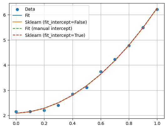
The intercept is the value of our output/target variable when all our features are zero and our function crosses the \(y\)-axis (for a one-dimensional case).
Printing the MSE, we see first that both methods give the same MSE, as they should. However, when we move to for example Ridge regression, the way we treat the intercept may give a larger or smaller MSE, meaning that the MSE can be penalized by the value of the intercept. Not including the intercept in the fit, means that the regularization term does not include \(\beta_0\). For different values of \(\lambda\), this may lead to different MSE values.
To remind the reader, the regularization term, with the intercept in Ridge regression, is given by
but when we take out the intercept, this equation becomes
For Lasso regression we have
It means that, when scaling the design matrix and the outputs/targets, by subtracting the mean values, we have an optimization problem which is not penalized by the intercept. The MSE value can then be smaller since it focuses only on the remaining quantities. If we however bring back the intercept, we will get a MSE which then contains the intercept.
Armed with this wisdom, we attempt first to simply set the intercept equal to False in our implementation of Ridge regression for our well-known vanilla data set.
import numpy as np
import pandas as pd
import matplotlib.pyplot as plt
from sklearn.model_selection import train_test_split
from sklearn import linear_model

def MSE(y_data,y_model):
    n = np.size(y_model)
    return np.sum((y_data-y_model)**2)/n


# A seed just to ensure that the random numbers are the same for every run.
# Useful for eventual debugging.
np.random.seed(3155)

n = 100
x = np.random.rand(n)
y = np.exp(-x**2) + 1.5 * np.exp(-(x-2)**2)

Maxpolydegree = 20
X = np.zeros((n,Maxpolydegree))
#We include explicitely the intercept column
for degree in range(Maxpolydegree):
    X[:,degree] = x**degree
# We split the data in test and training data
X_train, X_test, y_train, y_test = train_test_split(X, y, test_size=0.2)

p = Maxpolydegree
I = np.eye(p,p)
# Decide which values of lambda to use
nlambdas = 6
MSEOwnRidgePredict = np.zeros(nlambdas)
MSERidgePredict = np.zeros(nlambdas)
lambdas = np.logspace(-4, 2, nlambdas)
for i in range(nlambdas):
    lmb = lambdas[i]
    OwnRidgeBeta = np.linalg.pinv(X_train.T @ X_train+lmb*I) @ X_train.T @ y_train
    # Note: we include the intercept column and no scaling
    RegRidge = linear_model.Ridge(lmb,fit_intercept=False)
    RegRidge.fit(X_train,y_train)
    # and then make the prediction
    ytildeOwnRidge = X_train @ OwnRidgeBeta
    ypredictOwnRidge = X_test @ OwnRidgeBeta
    ytildeRidge = RegRidge.predict(X_train)
    ypredictRidge = RegRidge.predict(X_test)
    MSEOwnRidgePredict[i] = MSE(y_test,ypredictOwnRidge)
    MSERidgePredict[i] = MSE(y_test,ypredictRidge)
    print("Beta values for own Ridge implementation")
    print(OwnRidgeBeta)
    print("Beta values for Scikit-Learn Ridge implementation")
    print(RegRidge.coef_)
    print("MSE values for own Ridge implementation")
    print(MSEOwnRidgePredict[i])
    print("MSE values for Scikit-Learn Ridge implementation")
    print(MSERidgePredict[i])

# Now plot the results
plt.figure()
plt.plot(np.log10(lambdas), MSEOwnRidgePredict, 'r', label = 'MSE own Ridge Test')
plt.plot(np.log10(lambdas), MSERidgePredict, 'g', label = 'MSE Ridge Test')

plt.xlabel('log10(lambda)')
plt.ylabel('MSE')
plt.legend()
plt.show()
The results here agree when we force Scikit-Learn’s Ridge function to include the first column in our design matrix. We see that the results agree very well. Here we have thus explicitely included the intercept column in the design matrix. What happens if we do not include the intercept in our fit? Let us see how we can change this code by zero centering.
import numpy as np
import pandas as pd
import matplotlib.pyplot as plt
from sklearn.model_selection import train_test_split
from sklearn import linear_model
from sklearn.preprocessing import StandardScaler

def MSE(y_data,y_model):
    n = np.size(y_model)
    return np.sum((y_data-y_model)**2)/n
# A seed just to ensure that the random numbers are the same for every run.
# Useful for eventual debugging.
np.random.seed(315)

n = 100
x = np.random.rand(n)
y = np.exp(-x**2) + 1.5 * np.exp(-(x-2)**2)

Maxpolydegree = 20
X = np.zeros((n,Maxpolydegree-1))

for degree in range(1,Maxpolydegree): #No intercept column
    X[:,degree-1] = x**(degree)

# We split the data in test and training data
X_train, X_test, y_train, y_test = train_test_split(X, y, test_size=0.2)

#For our own implementation, we will need to deal with the intercept by centering the design matrix and the target variable
X_train_mean = np.mean(X_train,axis=0)
#Center by removing mean from each feature
X_train_scaled = X_train - X_train_mean
X_test_scaled = X_test - X_train_mean
#The model intercept (called y_scaler) is given by the mean of the target variable (IF X is centered)
#Remove the intercept from the training data.
y_scaler = np.mean(y_train)
y_train_scaled = y_train - y_scaler

p = Maxpolydegree-1
I = np.eye(p,p)
# Decide which values of lambda to use
nlambdas = 6
MSEOwnRidgePredict = np.zeros(nlambdas)
MSERidgePredict = np.zeros(nlambdas)

lambdas = np.logspace(-4, 2, nlambdas)
for i in range(nlambdas):
    lmb = lambdas[i]
    OwnRidgeBeta = np.linalg.pinv(X_train_scaled.T @ X_train_scaled+lmb*I) @ X_train_scaled.T @ (y_train_scaled)
    intercept_ = y_scaler - X_train_mean@OwnRidgeBeta #The intercept can be shifted so the model can predict on uncentered data
    #Add intercept to prediction
    ypredictOwnRidge = X_test_scaled @ OwnRidgeBeta + y_scaler
    RegRidge = linear_model.Ridge(lmb)
    RegRidge.fit(X_train,y_train)
    ypredictRidge = RegRidge.predict(X_test)
    MSEOwnRidgePredict[i] = MSE(y_test,ypredictOwnRidge)
    MSERidgePredict[i] = MSE(y_test,ypredictRidge)
    print("Beta values for own Ridge implementation")
    print(OwnRidgeBeta) #Intercept is given by mean of target variable
    print("Beta values for Scikit-Learn Ridge implementation")
    print(RegRidge.coef_)
    print('Intercept from own implementation:')
    print(intercept_)
    print('Intercept from Scikit-Learn Ridge implementation')
    print(RegRidge.intercept_)
    print("MSE values for own Ridge implementation")
    print(MSEOwnRidgePredict[i])
    print("MSE values for Scikit-Learn Ridge implementation")
    print(MSERidgePredict[i])


# Now plot the results
plt.figure()
plt.plot(np.log10(lambdas), MSEOwnRidgePredict, 'b--', label = 'MSE own Ridge Test')
plt.plot(np.log10(lambdas), MSERidgePredict, 'g--', label = 'MSE SL Ridge Test')
plt.xlabel('log10(lambda)')
plt.ylabel('MSE')
plt.legend()
plt.show()
We see here, when compared to the code which includes explicitely the intercept column, that our MSE value is actually smaller. This is because the regularization term does not include the intercept value \(\beta_0\) in the fitting. This applies to Lasso regularization as well. It means that our optimization is now done only with the centered matrix and/or vector that enter the fitting procedure.